Genetic Forward
Genetic Forward Modeling: the method
The method we refer to as Genetic Forward Modeling is built around a genetic algorithms, and functions as follows. Consider a model defined by a set of N parameters a={a_1,a_2,...a_N}, and a goodness-of-fit measure (or "fitness") f(a) computable for any given realization of the model. The task is to find the set of parameters a* corresponding to the model that maximizes f(a). A top-level view of a standard genetic algorithm for this task could be as follows:- Construct an initial random "population", i.e., a group of parameters sets a chosen completely randomly. Evaluate the fitness of each population member.
- Construct a new population by breeding selected individuals (selection based on fitness) from the old population.
- Evaluate fitness (i.e., calculate f(a)) for each member of the new population.
- Replace the old population by the new population.
- Repeat steps (2)---(4) until the fittest individual reaches or exceeds the desired goodness-of-fit level.
An important point to note is that the specific form of the relationship between f(a) and its defining parameters (linear vs nonlinear, etc.) does not affect the structure of the algorithm. f(a) need not even be differentiable with respect to the defining parameters, as no gradient information is required by the algorithm.
All results discussed under this page were obtained using the genetic algorithm-based general purpose optimization FORTRAN subroutine PIKAIA. This subroutine is public domain software and is available electronically on anonymous ftp from the High Altitude Observatory.
Application to helioseismology
Genetic Forward modeling applied to helioseismic inversion of the Sun's internal differential rotation is carried out as follows. The data consists of a discrete set of frequency splittings a*(n,l,s) with associated errors epsilon_nls. The data is related to the internal rotation profile through the following integral equation:
which expresses the fact that the measured frequency splitting for a pair of prograde/retrograde modes of identical radial degree n and angular degree l is a global measure of the rotation rate encountered by the mode as it travels through the solar interior. A solar structural model is assumed given so that the integration Kernels K(a)_nls are known quantities. The solution procedure is a direct transcription of the general genetic forward modeling algorithm outlined previously:
2-D inversion of p-mode data: the solar tachocline
As part of an ongoing group effort aimed at evaluating the depth and thickness of the rotational transition layer at the base of the solar convection zone (the tachocline), genetic forward modeling was used in conjunction with the following parametrization of the solar internal rotation profile: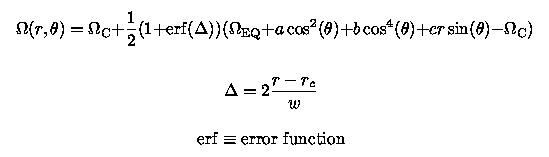
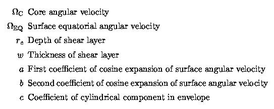
r_c=0.705 +/- 0.002
w=0.053 +/- 0.015
The rotation rate of the deep solar core
The same genetic forward modeling technique has been used to perform 1-D reconstructions of the rotation rate in the deep part of the solar radiative core. With the rotation rate assumed given in r/R=0.5, a 1-D rotation curve is defined on a discrete spatial mesh, assuming piecewise linear variations between mesh points. The nodal values are then treated as fitting parameters by the genetic algorithm. A total of 203 modes are used, with angular degree l in the range 1-24, and radial degree n in the range 10-24. All these modes have their inner turning point below r/R=0.5. The chi^2 is computed in terms of the first three splitting coefficients a1, a3 and a5. Modeling results indicate that the solar code rotates essentially rigidly at least down to r/R=0.2, and rule out increases by more than a factor of two down to r/R=0.1: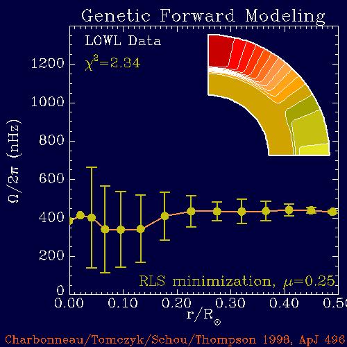
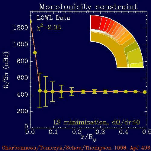
Regularized least-squares solution obtained by genetic forward modeling. The error bars have been estimated by Monte Carlo simulations on synthetic datasets. The inset shows the parametric, solar-like rotation profile used above r/R=0.5, with contour spacing of 10nHz. These results have been shown to be robust with respect to the various modeling assumptions, including the choice of frequency splitting modeset, rotation profile above r/R=0.5, of regularization constraint, of one-dimensionality, and of statistical estimator being minimized (as discussed in the 1998 paper by Charbonneau et al. listed below). In particular, we use a monotonicity constraint that, unlike the smoothing functionals commonly used in regularized least-squares approaches, does not assign any penalty to any inward increase in rotation rate. We can thus rule out the possibility that the flat rotation curve shown above is a mere consequence of the smoothness constraint used in conjunction with the least-squares estimator. The genetic algorithm-based method largely outperforms standard Monte Carlo techniques, in the sense that far, far fewer model evaluations are needed to obtained a model yieldling a good fit. The Figure below shows such a comparison, carried out for synthetic data using a monotonicity-constrained least-squares technique. Each thick curve is an average of 20 runs, and so should be reasonably representative of the true performance of each method. The thinner lines The red error bar corresponds to the range of Monte Carlo solutions after 2000 generations (100000 model evaluations).
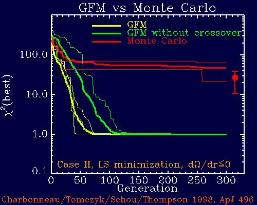
Convergence curves for genetic forward modeling (yellow), and basic Monte Carlo technique (red). To allow equitable comparison between both methods, one generation also corresponds to 50 model evaluations for the Monte Carlo technique. Each curve is an average of 20 runs, and the thin lines are the slowest and fastest converging solutions (normalized chi^2 less than 2) for both methods. The green line is genetic forward modeling convergence curve obtained using identical parameter settings as for the yellow line, with the single exception that the crossover operator has been turned off within the genetic algorithm
Publications:
Tomczyk, S., Charbonneau, P. Schou, J., and Thompson, M.J. 1995, Constraining solar core rotation with genetic forward modeling in Proceedings of the fourth SOHO Workshop: Helioseismology, ESA SP-376, 271-274. [paper] Charbonneau, P., Christensen-Dalsgaard, J., Henning, R., Schou, J., Tomczyk, S., and Thompson, M.J. 1996, Observational constraints on the dynamical properties of the shear layer at the base of the solar convection zone, in IAU Symp. 181: Sounding solar and stellar interiors (Poster volume, eds. J.~Provost & F.-X. Schmider, 161-162, 1998). [paper]. Charbonneau, P., Tomczyk, S. 1997, Helioseismology by Genetic Forward Modeling, in 12th Kingston meeting: Computational Astrophysics, ASP Conference Series vol. 123, eds. D.A. Clarke and M.J. West, 49-54. [reprint] Charbonneau, P., Tomczyk, S., Schou, J., and Thompson, M.J. 1998, The rotation of the solar core inferred by genetic forward modeling, in The Astrophysical Journal, vol. 496, 1015-1030. [Abstract]
Application to coronal modeling
The bright coronal structures known as helmet streamers, so spectacularly obvious at times of total solar eclipses own their existence to the confining effect of large-scale, closed magnetic structures anchored in the solar photosphere. While the solar magnetic field cannot yet be directly measured in the corona, quantitative information regarding its geometry and strength can be obtained by fitting to observed coronal brightness distribution a model that yields self-consistently both the density and magnetic field distributions. This modeling task is most easily carried out on the solar minimum corona. At time of activity minimum the corona is characterized by an axisymmetric structure, with a belt of streamers straddling the equator and large coronal holes over polar regions. The observable being fit is the so-called polarization brightness (pB) in the plane of the sky, which is related to the underlying density distribution through the following integral relation:
where the integral is carried over the line-of-sight (los), and the electron density (ne) is a function of spatial coordinates and of the set a of model parameters being adjusted to minimize the chi^2 of the model pB with respect to the observed pB. This parameter adjustment is readily carried out by genetic forward modeling.
Publications:
Gibson, S.E., and Charbonneau, P. 1997, Empirical modeling of the solar corona using genetic algorithms, J. Geophys. Res., 103(A7), 14511-14521. [abstract]