Saving Diagnostic Fields
The diagnostics module (diags.F) in the TIEGCM will calculate and save diagnostic fields to the secondary histories. The user can add any subset of these fields to the SECFLDS parameter list in the namelist input file. See the diagnostics namelist example.
Table of Available Diagnostics
Following is a table of diagnostic fields that can be saved on secondary histories by including the short names in the SECFLDS namelist input parameter. Click on the short name to obtain detailed information about the calculation and saving of a diagnostic field.
On the history files, “Short Name” will be the variable name, and “Long Name” and “Units” will be attributes of the variable. “Grid” refers to the number of dimensions (2d lat-lon, or 3d lat-lon-level), and whether the field is on the geographic or geomagnetic grid.
A text version of the table is also available, and is printed to stdout by a model run (ordering of the fields in the text table may be different than in the below table).
| Short Name | Long Name | Units | Grid |
|---|---|---|---|
| CO2_COOL | CO2 Cooling | erg/g/s | 3d geo |
| NO_COOL | NO Cooling | erg/g/s | 3d geo |
| DEN | Total Neutral Density | g/cm3 | 3d geo |
| HEATING | Total Heating | erg/g/s | 3d geo |
| SCHT | Pressure Scale Height | km | 3d geo |
| SIGMA_HAL | Hall Conductivity | S/m | 3d geo |
| SIGMA_PED | Pedersen Conductivity | S/m | 3d geo |
| LAMDA_HAL | Hall Ion Drag Coefficient | 1/s | 3d geo |
| LAMDA_PED | Pedersen Ion Drag Coefficient | 1/s | 3d geo |
| UI_ExB | Zonal Ion Drift | cm/s | 3d geo |
| VI_ExB | Meridional Ion Drift | cm/s | 3d geo |
| WI_ExB | Vertical Ion Drift | cm/s | 3d geo |
| MU_M | Molecular Viscosity Coefficient | g/cm/s | 3d geo |
| WN | Neutral Vertical Wind | cm/s | 3d geo |
| O_N2 | O/N2 Ratio | [none] | 3d geo |
| QJOULE | Joule Heating | erg/g/s | 3d geo |
| QJOULE_INTEG | Height-integrated Joule Heating | erg/cm2/s | 2d geo |
| HMF2 | Height of the F2 Layer | km | 2d geo |
| NMF2 | Peak Density of the F2 Layer | 1/cm3 | 2d geo |
| TEC | Total Electron Content | 1/cm2 | 2d geo |
| JE13D | Eastward current density (3d) | A/m2 | 3d mag |
| JE23D | Downward current density (3d) | A/m2 | 3d mag |
| JQR | Upward current density (2d) | A/m2 | 2d mag |
| KQLAM | Height-integ current density (+north) | A/m | 2d mag |
| KQPHI | Height-integ current density (+east) | A/m | 2d mag |
Saving Fields/Arrays from the Source Code
In addition to the “sanctioned” diagnostics, arbitrary 2d and 3d arrays can be saved from the model to secondary histories by inserting a call to subroutine addfld (addfld.F) in the source code. (See the chapter on Modifying Source Code in this document for information about modifying the source code.) There are many examples of this in the source code, just grep on “call addfld”. For more information about how to make calls to addfld, please see comments in the addfld.F source file.
Here are a couple of examples of addfld calls from near the end of subroutine qrj (qrj.F). These calls are inside a latitude loop, where the loop variable index is “lat”. Normally, in parallel code, subdomains of the field are passed, e.g., lon0:lon1 and lat0:lat1:
 call addfld('QO2P'  ,' ',' ',  qo2p(lev0:lev1,lon0:lon1,lat),
|  'lev',lev0,lev1,'lon',lon0,lon1,lat)
 call addfld('QN2P'  ,' ',' ',  qn2p(lev0:lev1,lon0:lon1,lat),
|  'lev',lev0,lev1,'lon',lon0,lon1,lat)
 call addfld('QNP'   ,' ',' ',   qnp(lev0:lev1,lon0:lon1,lat),
|  'lev',lev0,lev1,'lon',lon0,lon1,lat)
The calling sequence for subroutine addfld is explained in comments at the top of source file addfld.F.
Details of Diagnostic Field Calculations
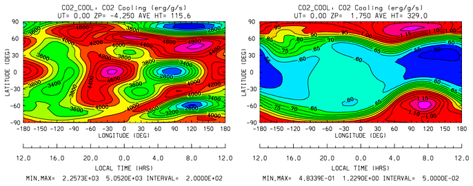
- CO2_COOL
Diagnostic field: CO2 Cooling (erg/g/s):
diags(n)%short_name = 'CO2_COOL'
diags(n)%long_name  = 'CO2 Cooling'
diags(n)%units      = 'erg/g/s'
diags(n)%levels     = 'lev'
diags(n)%caller     = 'newton.F'
This field is calculated in newton.F and passed to mkdiag_CO2COOL (diags.F), where it is saved to the secondary history. The calculation of CO2 cooling in newton.F is as follows:
     co2_cool(k,i) = 2.65e-13*nco2(k,i)*exp(-960./tn(k,i))*
|      avo*((o2(k,i)*rmassinv_o2+(1.-o2(k,i)-o1(k,i))*rmassinv_n2)*
|      aco2(k,i)+o1(k,i)*rmassinv_o1*bco2(k,i))
Sample images: CO2_COOL Global maps at Zp -4, +2:
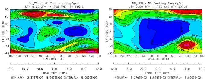
- NO_COOL
Diagnostic field: NO Cooling (erg/g/s):
diags(n)%short_name = 'NO_COOL'
diags(n)%long_name  = 'NO Cooling'
diags(n)%units      = 'erg/g/s'
diags(n)%levels     = 'lev'
diags(n)%caller     = 'newton.F'
This field is calculated in newton.F and passed to mkdiag_NOCOOL (diags.F), where it is saved to the secondary history. The calculation of NO cooling in newton.F is as follows:
     no_cool(k,i) = 4.956e-12*(avo*no(k,i)*rmassinv_no)*
|      (ano(k,i)/(ano(k,i)+13.3))*exp(-2700./tn(k,i))
Sample images: NO_COOL Global maps at Zp -4, +2:
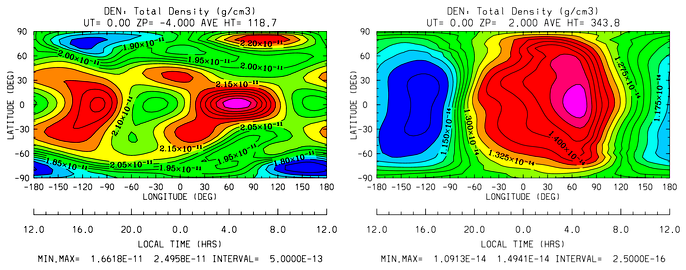
- DEN
Diagnostic field: Total Density (g/cm3):
diags(n)%short_name = 'DEN'
diags(n)%long_name  = 'Total Density'
diags(n)%units      = 'g/cm3'
diags(n)%levels     = 'ilev'
diags(n)%caller     = 'dt.F'
This field is calculated in dt.F and passed to mkdiag_DEN (diags.F), where it is saved to the secondary history. The calculation of DEN (rho) in dt.F is as follows:
do i=lon0,lon1
  do k=lev0+1,lev1-1
    tni(k,i) = .5*(tn(k-1,i,lat)+tn(k,i,lat))
    h(k,i) = gask*tni(k,i)/barm(k,i,lat)
    rho(k,i) = p0*expzmid_inv*expz(k)/h(k,i)
  enddo ! k=lev0+1,lev1-1
  rho(lev0,i) = p0*expzmid_inv*expz(lev0)/h(lev0,i)
  rho(lev1,i) = p0*expzmid*expz(lev1-1)/h(lev1,i)
enddo ! i=lon0,lon1
Sample images: DEN Global maps at Zp -4, +2:
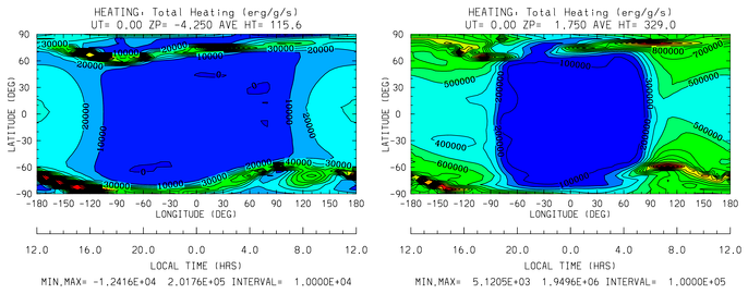
- HEATING
Diagnostic field: Total Heating (erg/g/s):
diags(n)%short_name = 'HEATING'
diags(n)%long_name  = 'Total Heating'
diags(n)%units      = 'erg/g/s'
diags(n)%levels     = 'lev'
diags(n)%caller     = 'dt.F'
This field is calculated in dt.F and passed to mkdiag_HEAT (diags.F), where it is saved to the secondary history. The calculation of HEATING (rho) in dt.F sums the following heat sources:
- Total solar heating (see qtotal in qrj.F)
- Heating from 4th order horizontal diffusion
- Heating due to atomic oxygen recombination
- Ion Joule heating
- Heating due to molecular diffusion
Sample images: HEATING Global maps at Zp -4, +2:
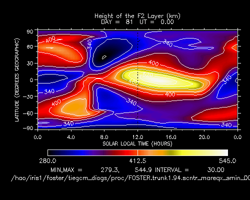
- HMF2
Diagnostic field (2d lat x lon): Height of the F2 Layer (km):
diags(n)%short_name = 'HMF2'
diags(n)%long_name  = 'Height of the F2 Layer'
diags(n)%units      = 'km'
diags(n)%levels     = 'none' ! hmf2 is 2d lon x lat
diags(n)%caller     = 'elden.F'
The height of the F2 layer is calculated and saved by subroutines mkdiag_HNMF2 and hnmf2 in source file diags.F.
Sub mkdiag_HNMF2 is called by subroutine elden in source file elden.F, as follows:
call mkdiag_HNMF2(‘HMF2’,z,electrons,lev0,lev1,lon0,lon1,lat)Note
Occaisionally this algorithm will return the peak electron density in the E-region, instead of the F-region, in small areas of the global domain, usually at high latitide. This can result in pockets of anonymously low values for HMF2, e.g., around 125 km.
Sample images: HMF2 Global map:
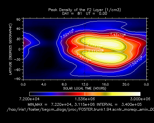
- NMF2
Diagnostic field (2d lat x lon): Peak Density of the F2 Layer (1/cm3):
diags(n)%short_name = 'NMF2'
diags(n)%long_name  = 'Peak Density of the F2 Layer'
diags(n)%units      = '1/cm3'
diags(n)%levels     = 'none' ! nmf2 is 2d lon x lat
diags(n)%caller     = 'elden.F'
The peak density of the the F2 layer is calculated and saved by subroutines mkdiag_HNMF2 and hnmf2 in source file diags.F.
Sub mkdiag_HNMF2 is called by subroutine elden in source file elden.F, as follows:
call mkdiag_HNMF2(‘NMF2’,z,electrons,lev0,lev1,lon0,lon1,lat)Sample images: NMF2 Global map:
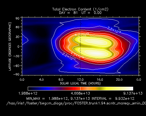
- TEC
Diagnostic field (2d lat x lon): Total Electron Content (1/cm2):
diags(n)%short_name = 'TEC'
diags(n)%long_name  = 'Total Electron Content'
diags(n)%units      = '1/cm2'
diags(n)%levels     = 'none' ! 2d lon x lat
diags(n)%caller     = 'elden.F'
Total Electron Content is calculated by subroutine mkdiag_TEC in source file diags.F, as follows:
!
! Integrate electron content in height at current latitude:
      tec(:) = 0.
      do i=lon0,lon1
        do k=lev0,lev1-1
          tec(i) = tec(i)+(z(k+1,i)-z(k,i))*electrons(k,i)
        enddo
      enddo
Subroutine mkdiags_TEC is called by subroutine elden in source file elden.F as follows:
call mkdiag_TEC('TEC',tec,z,electrons,lev0,lev1,lon0,lon1,lat)Sample images: TEC Global map
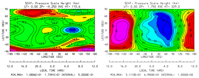
- SCHT
Diagnostic field: Pressure Scale Height (km):
diags(n)%short_name = 'SCHT'
diags(n)%long_name  = 'Pressure Scale Height'
diags(n)%units      = 'km'
diags(n)%levels     = 'lev'
diags(n)%caller     = 'addiag.F'
The Pressure Scale Height is calculated from the geopotential and saved by subroutine mkdiag_SCHT in source file diags.F. This code summarizes the calculation:
!
! Take delta Z:
      do j=lat0,lat1
        do i=lon0,lon1
          do k=lev0,lev1-1
            pzps(k,i) = zcm(k+1,i,j)-zcm(k,i,j)
          enddo
          pzps(lev1,i) = pzps(lev1-1,i)
!
! Generic for dlev 0.5 or 0.25 resolution:
          pzps(:,i) = pzps(:,i)/dlev
        enddo ! i=lon0,lon1
        pzps = pzps*1.e-5 ! cm to km
      enddo ! j=lat0,lat1
Subroutine mkdiag_SCHT is called from subroutine addiag (source file addiag.F).
Sample images: SCHT Global maps at Zp -4, +2:
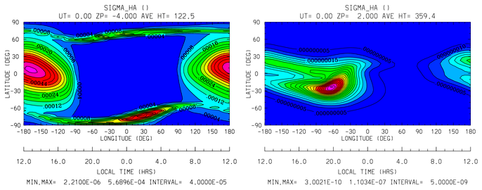
- SIGMA_HAL
Diagnostic field: Hall Conductivity (S/m):
diags(n)%short_name = 'SIGMA_HAL'
diags(n)%long_name  = 'Hall Conductivity'
diags(n)%units      = 'S/m'
diags(n)%levels     = 'lev'
diags(n)%caller     = 'lamdas.F'
The Hall Conductivity is calculated by subroutine lamdas (source file lamdas.F), and passed to sub mkdiag_SIGMAHAL (diags.F), where it is saved to secondary histories. The calculation in lamdas.F is summarized as follows:
! Pedersen and Hall conductivities (siemens/m):
! Qe_fac includes conversion from CGS to SI units
!  -> e/B [C/T 10^6 m^3/cm^3], see above.
! number densities [1/cm^3]
!
      do i=lon0,lon1
        do k=lev0,lev1-1
!
! ne = electron density assuming charge equilibrium [1/cm3]:
          ne(k,i) = op(k,i)+o2p(k,i)+nop(k,i)
!
! Hall conductivity [S/m] (half level):
          sigma_hall(k,i) = qe_fac(i)*
|           (ne (k,i)/(1.+rnu_ne (k,i)**2)-
|            op (k,i)/(1.+rnu_op (k,i)**2)-
|            o2p(k,i)/(1.+rnu_o2p(k,i)**2)-
|            nop(k,i)/(1.+rnu_nop(k,i)**2))
        enddo ! k=lev0,lev1-1
      enddo ! i=lon0,lon1
Sample images: SIGMA_HAL Global maps at Zp -4, +2:
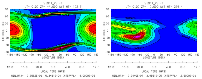
- SIGMA_PED
Diagnostic field: Pedersen Conductivity (S/m):
diags(n)%short_name = 'SIGMA_PED'
diags(n)%long_name  = 'Pedersen Conductivity'
diags(n)%units      = 'S/m'
diags(n)%levels     = 'lev'
diags(n)%caller     = 'lamdas.F'
The Pedersen Conductivity is calculated by subroutine lamdas (source file lamdas.F), and passed to sub mkdiag_SIGMAPED (diags.F), where it is saved to secondary histories. The calculation in lamdas.F is summarized as follows:
! Pedersen and Hall conductivities (siemens/m):
! Qe_fac includes conversion from CGS to SI units
!  -> e/B [C/T 10^6 m^3/cm^3], see above.
! number densities [1/cm^3]
!
      do i=lon0,lon1
        do k=lev0,lev1-1
!
! ne = electron density assuming charge equilibrium [1/cm3]:
          ne(k,i) = op(k,i)+o2p(k,i)+nop(k,i)
!
! Pedersen conductivity [S/m] (half level):
          sigma_ped(k,i) = qe_fac(i)*
     |      ((op (k,i)*rnu_op (k,i)/(1.+rnu_op (k,i)**2))+
     |       (o2p(k,i)*rnu_o2p(k,i)/(1.+rnu_o2p(k,i)**2))+
     |       (nop(k,i)*rnu_nop(k,i)/(1.+rnu_nop(k,i)**2))+
     |       (ne (k,i)*rnu_ne (k,i)/(1.+rnu_ne (k,i)**2)))
        enddo ! k=lev0,lev1-1
      enddo ! i=lon0,lon1
Sample images: SIGMA_PED Global maps at Zp -4, +2:
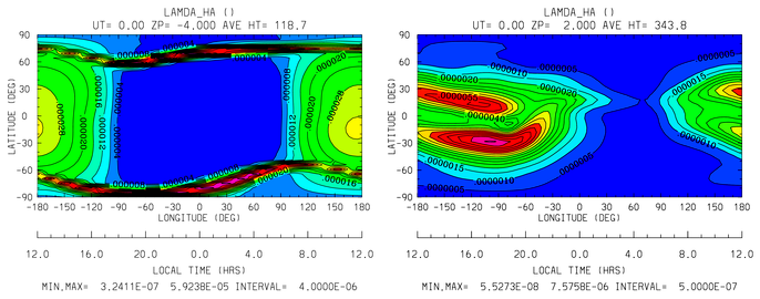
- LAMDA_HAL
Diagnostic field: Hall Ion Drag Coefficient (1/s):
diags(n)%short_name = 'LAMDA_HAL'
diags(n)%long_name  = 'Hall Ion Drag Coefficient'
diags(n)%units      = '1/s'
diags(n)%levels     = 'lev'
diags(n)%caller     = 'lamdas.F'
The Hall Ion Drag Coefficient is calculated in subroutine lamdas (source file lamdas.F), and saved to seconday histories by subroutine mkdiag_LAMDAHAL (diags.F).
Sample images: LAMDA_HAL Global maps at Zp -4, +2:
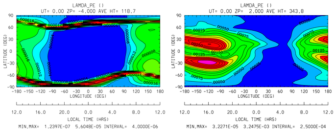
- LAMDA_PED
Diagnostic field: Hall Ion Drag Coefficient (1/s):
diags(n)%short_name = 'LAMDA_PED'
diags(n)%long_name  = 'Pedersen Ion Drag Coefficient'
diags(n)%units      = '1/s'
diags(n)%levels     = 'lev'
diags(n)%caller     = 'lamdas.F'
The Pedersen Ion Drag Coefficient is calculated in subroutine lamdas (source file lamdas.F), and saved to secondary histories by subroutine mkdiag_LAMDAPED (diags.F).
Sample images: LAMDA_PED Global maps at Zp -4, +2:
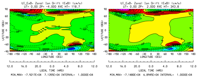
- UI_ExB
Diagnostic field: Zonal Ion Drift (ExB) (cm/s):
diags(n)%short_name = 'UI_ExB'
diags(n)%long_name  = 'Zonal Ion Drift (ExB)'
diags(n)%units      = 'cm/s'
diags(n)%levels     = 'ilev'
diags(n)%caller     = 'ionvel.F'
Calculated by subroutine ionvel (ionvel.F):
!
! ion velocities = (e x b/b**2)
! ui = zonal, vi = meridional, wi = vertical
        do k=lev0,lev1
          do i=lonbeg,lonend
            ui(k,i,lat) = -(eey(k,i)*zb(i-2,lat)+eez(k,i)*xb(i-2,lat))*
|             1.e6/bmod(i-2,lat)**2
            vi(k,i,lat) =  (eez(k,i)*yb(i-2,lat)+eex(k,i)*zb(i-2,lat))*
|             1.e6/bmod(i-2,lat)**2
            wi(k,i,lat) =  (eex(k,i)*xb(i-2,lat)-eey(k,i)*yb(i-2,lat))*
|             1.e6/bmod(i-2,lat)**2
          enddo ! i=lon0,lon1
        enddo ! k=lev0,lev1
Subroutine ionvel calls subroutine mkdiag_UI (diags.F) to save the field to secondary histories. The field is converted from m/s to cm/s in ionvel before the call to mkdiag_UI.
Sample images: UI_ExB Global maps at Zp -4, +2:
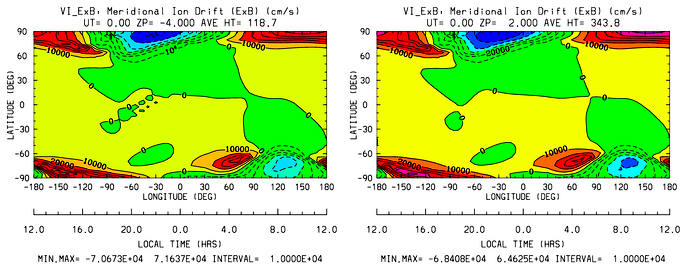
- VI_ExB
Diagnostic field: Meridional Ion Drift (ExB) (cm/s):
diags(n)%short_name = 'VI_ExB'
diags(n)%long_name  = 'Meridional Ion Drift (ExB)'
diags(n)%units      = 'cm/s'
diags(n)%levels     = 'ilev'
diags(n)%caller     = 'ionvel.F'
Calculated by subroutine ionvel (ionvel.F):
!
! ion velocities = (e x b/b**2)
! ui = zonal, vi = meridional, wi = vertical
        do k=lev0,lev1
          do i=lonbeg,lonend
            ui(k,i,lat) = -(eey(k,i)*zb(i-2,lat)+eez(k,i)*xb(i-2,lat))*
|             1.e6/bmod(i-2,lat)**2
            vi(k,i,lat) =  (eez(k,i)*yb(i-2,lat)+eex(k,i)*zb(i-2,lat))*
|             1.e6/bmod(i-2,lat)**2
            wi(k,i,lat) =  (eex(k,i)*xb(i-2,lat)-eey(k,i)*yb(i-2,lat))*
|             1.e6/bmod(i-2,lat)**2
          enddo ! i=lon0,lon1
        enddo ! k=lev0,lev1
Subroutine ionvel calls subroutine mkdiag_VI (diags.F) to save the field to secondary histories. The field is converted from m/s to cm/s in ionvel before the call to mkdiag_VI.
Sample images: VI_ExB Global maps at Zp -4, +2:
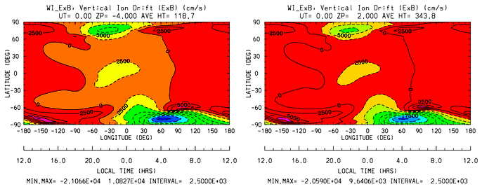
- WI_ExB
Diagnostic field: Vertical Ion Drift (ExB) (cm/s):
diags(n)%short_name = 'WI_ExB'
diags(n)%long_name  = 'Vertical Ion Drift (ExB)'
diags(n)%units      = 'cm/s'
diags(n)%levels     = 'ilev'
diags(n)%caller     = 'ionvel.F'
Calculated by subroutine ionvel (ionvel.F):
!
! ion velocities = (e x b/b**2)
! ui = zonal, vi = meridional, wi = vertical
        do k=lev0,lev1
          do i=lonbeg,lonend
            ui(k,i,lat) = -(eey(k,i)*zb(i-2,lat)+eez(k,i)*xb(i-2,lat))*
|             1.e6/bmod(i-2,lat)**2
            vi(k,i,lat) =  (eez(k,i)*yb(i-2,lat)+eex(k,i)*zb(i-2,lat))*
|             1.e6/bmod(i-2,lat)**2
            wi(k,i,lat) =  (eex(k,i)*xb(i-2,lat)-eey(k,i)*yb(i-2,lat))*
|             1.e6/bmod(i-2,lat)**2
          enddo ! i=lon0,lon1
        enddo ! k=lev0,lev1
Subroutine ionvel calls subroutine mkdiag_UI (diags.F) to save the field to secondary histories. The field is converted from m/s to cm/s in ionvel before the call to mkdiag_WI.
Sample images: WI_ExB Global maps at Zp -4, +2:
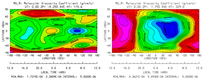
- MU_M
Diagnostic field: Molecular Viscosity Coefficient (g/cm/s):
diags(n)%short_name = 'MU_M'
diags(n)%long_name  = 'Molecular Viscosity Coefficient'
diags(n)%units      = 'g/cm/s'
diags(n)%levels     = 'lev'
diags(n)%caller     = 'cpktkm.F'
The Molecular Viscosity Coefficient is calculated by subroutine cpktkm (source file cpktkm.F), and saved to secondary histories by subroutine mkdiag_MU_M (diags.F). The calculation in cpktkm is summarized as follows:
fkm(k,i) = po2(k,i)*4.03 + pn2(k,i)*3.42 + po1(k,i)*3.9
Sample images: MU_M Global maps at Zp -4, +2:
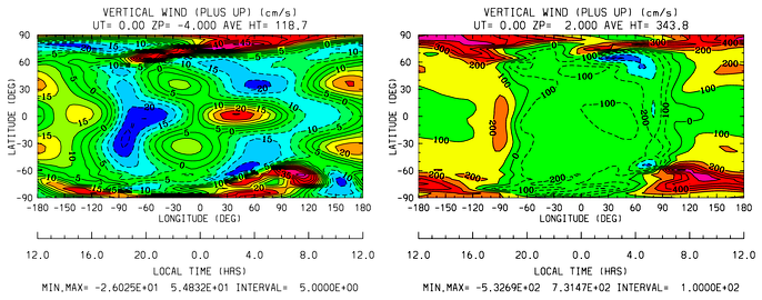
- WN
Diagnostic field: Neutral Vertical Wind (cm/s):
diags(n)%short_name = 'WN'
diags(n)%long_name  = 'NEUTRAL VERTICAL WIND (plus up)'
diags(n)%units      = 'cm/s'
diags(n)%levels     = 'ilev'
diags(n)%caller     = 'swdot.F'
Note
This 3d field is calculated on fixed pressure surfaces ln(p0/p), i.e., there is no interpolation to height.
Calculated from OMEGA (vertical motion) and pressure scale height by subroutine mkdiag_WN in source file diags.F:
!-----------------------------------------------------------------------
      subroutine mkdiag_WN(name,omega,zcm,lev0,lev1,lon0,lon1,lat)
!
! Neutral Vertical Wind, from vertical motion OMEGA and scale height.
! Scale height pzps is calculated from input geopotential z (cm).
!
! Args:
      character(len=*),intent(in) :: name
      integer,intent(in) :: lev0,lev1,lon0,lon1,lat
      real,intent(in),dimension(lev0:lev1,lon0:lon1) :: omega,zcm
!
! Local:
      integer :: i,k,ix
      real,dimension(lev0:lev1,lon0:lon1) :: wn
      real,dimension(lev0:lev1) :: pzps,omega1
!
! Check that field name is a diagnostic, and was requested:
      ix = checkf(name) ; if (ix==0) return
!
! Calculate scale height pzps:
      do i=lon0,lon1
        do k=lev0+1,lev1-1
          pzps(k) = (zcm(k+1,i)-zcm(k-1,i))/(2.*dlev)
        enddo
        pzps(lev0) = (zcm(lev0+1,i)-zcm(lev0,i))/dlev
        pzps(lev1) = pzps(lev1-1)
!
        omega1(:) = omega(:,i)
        omega1(lev1) = omega1(lev1-1)
!
! Output vertical wind (cm):
        wn(:,i) = omega1(:)*pzps(:)
      enddo ! i=lon0,lon1

      call addfld(diags(ix)%short_name,diags(ix)%long_name,
     |  diags(ix)%units,wn,'lev',lev0,lev1,'lon',lon0,lon1,lat)

      end subroutine mkdiag_WN
!-----------------------------------------------------------------------
Called by: subroutine swdot in source file swdot.F as follows:
do lat=lat0,lat1
  call mkdiag_WN('WN',w(:,lon0:lon1,lat),z(:,lon0:lon1,lat),lev0,lev1,lon0,lon1,lat)
enddo
Sample images: WN Global maps at Zp -4, +2:
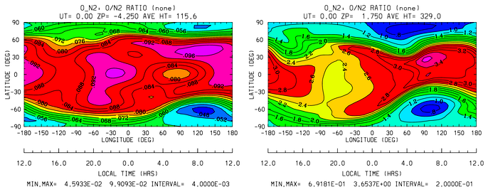
- O_N2
Diagnostic field: O/N2 RATIO:
diags(n)%short_name = 'O_N2'
diags(n)%long_name  = 'O/N2 RATIO'
diags(n)%units      = ' '
diags(n)%levels     = 'lev'
diags(n)%caller     = 'comp.F'
Note
Please note that this field is calculated at constant pressure surfaces (ln(p0/p)), and is very sensitive to fluctuations in the height of the pressure surfaces. If this field is interpolated to constant height surfaces, it will look very different than when plotted on pressure surfaces.
Note
Also note that O/N2 is a 3d field (not integrated in the vertical coordinate), and is the quotient of the mixing ratios of the species (i.e., there is no units conversion from MMR).
O/N2 is calculated and saved by subroutine mkdiag_O_N2 in source file diags.F:
!-----------------------------------------------------------------------
      subroutine mkdiag_O_N2(name,o1,o2,lev0,lev1,lon0,lon1,lat)
!
! Calculate O/N2 ratio from o2 and o (mmr).
! In mass mixing ratio, this is simply o/(1-o2-o)
!
! Args:
      character(len=*),intent(in) :: name
      integer,intent(in) :: lev0,lev1,lon0,lon1,lat
      real,intent(in),dimension(lev0:lev1,lon0:lon1) :: o1,o2
!
! Local:
      integer :: ix
      real,dimension(lev0:lev1,lon0:lon1) :: n2, o_n2
!
! Check that field name is a diagnostic, and was requested:
      ix = checkf(name) ; if (ix==0) return
!
! N2 mmr:
      n2 = 1.-o2-o1
!
! O/N2 ratio:
      o_n2 = o1/n2

      call addfld(diags(ix)%short_name,diags(ix)%long_name,
     |  diags(ix)%units,o_n2,'lev',lev0,lev1,'lon',lon0,lon1,lat)

      end subroutine mkdiag_O_N2
!-----------------------------------------------------------------------
Called by: subroutine comp in source file comp.F as follows:
   call mkdiag_O_N2('O_N2',o1_upd(:,lon0:lon1,lat),
|    o2_upd(:,lon0:lon1,lat),lev0,lev1,lon0,lon1,lat)
Sample images: O_N2 Global maps at Zp -4, +2:
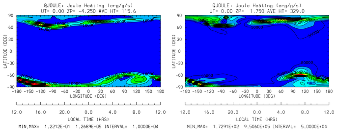
- QJOULE
Diagnostic field: Joule Heating (erg/g/s):
diags(n)%short_name = 'QJOULE'
diags(n)%long_name  = 'Joule Heating'
diags(n)%units      = 'erg/g/s'
diags(n)%levels     = 'lev'
diags(n)%caller     = 'qjoule.F'
Total Joule Heating is calculated in source file qjoule.F as qji_tn, and is passed to subroutine mkdiag_QJOULE (diags.F), where it is saved to secondary histories. The following code summarizes the calculation in qjoule.F:
 do i=lon0,lon1
   do k=lev0,lev1-1
     scheight(k,i) = gask*tn(k,i)/
|        (.5*(barm(k,i)+barm(k+1,i))*grav)
     vel_zonal(k,i) = .5*(ui(k,i)+ui(k+1,i))-un(k,i)  ! s2
     vel_merid(k,i) = .5*(vi(k,i)+vi(k+1,i))-vn(k,i)  ! s3
     vel_vert(k,i)  = .5*(wi(k,i)+wi(k+1,i)-scheight(k,i)*
|         ( w(k,i)-w(k+1,i)) )
   enddo ! k=lev0,lev1-1
 enddo ! i=lon0,lon1
 do i=lon0,lon1
   do k=lev0,lev1-1
     qji_tn(k,i) = .5*(lam1(k,i)+lam1(k+1,i))*
|      (vel_zonal(k,i)**2 + vel_merid(k,i)**2 +
|       vel_vert(k,i)**2)
   enddo ! k=lev0,lev1-1
 enddo ! i=lon0,lon1

 call mkdiag_QJOULE('QJOULE',qji_tn,lev0,lev1,lon0,lon1,lat)
Sample images: QJOULE Global maps at Zp -4, +2:
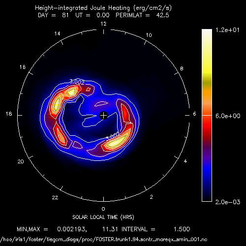
- QJOULE_INTEG
Diagnostic field: Height-integrated Joule Heating (W/m^2):
diags(n)%short_name = 'QJOULE_INTEG'
diags(n)%long_name  = 'Height-integrated Joule Heating'
diags(n)%units      = 'erg/cm2/s'
diags(n)%levels     = 'none'
diags(n)%caller     = 'qjoule.F'
Note
This field is integrated on pressure surfaces (not height), so is a 2d field. Also note it is first calculated in W/m^2, then converted to erg/g/cm2, for consistency with the model. See comment below if you would like the field to be returned in W/m^2.
Calculated and saved by subroutine mkdiag_QJOULE_INTEG in source file diags.F:
!-----------------------------------------------------------------------
      subroutine mkdiag_QJOULE_INTEG(name,qji_tn,lev0,lev1,lon0,lon1,
     |  lat)
      use cons_module,only: p0,grav
      use init_module,only: zpint
!
! Calculate height-integrated Joule heating (called from qjoule.F)
! This method is adapted from ncl code provided by Astrid (7/20/11)
!
! Args
      character(len=*),intent(in) :: name
      integer,intent(in) :: lev0,lev1,lon0,lon1,lat
      real,intent(in),dimension(lev0:lev1,lon0:lon1) :: qji_tn
!
! Local:
      integer :: ix,k,i
      real,dimension(lon0:lon1) :: qji_integ
      real,dimension(lev0:lev1,lon0:lon1) :: qj
      real :: myp0,mygrav
!
! Check that field name is a diagnostic, and was requested:
      ix = checkf(name) ; if (ix==0) return
!
! First integrate to get MKS units W/m^2:
! (If you want these units, comment out the below conversion to CGS)
!
      mygrav = grav*.01     ! cm/s^2 to m/s^2
      myp0 = p0*1.e-3*100.  ! to Pa
      qj = qji_tn*.0001     ! ergs/g/s to W/kg 10^(-7)*10^3

      qji_integ = 0.
      do i=lon0,lon1
        do k=lev0,lev1-1
          qji_integ(i) = qji_integ(i) + myp0/mygrav*exp(-zpint(k))*
     |      qj(k,i)*dlev
        enddo
      enddo
!
! Output in CGS units, to be consistent w/ the model:
! (note that 1 erg/cm^2/s == 1 mW/m^2)
      qji_integ = qji_integ*1000. ! W/m^2 to erg/cm^2/s
!
! Save 2d field on secondary history:
      call addfld(diags(ix)%short_name,diags(ix)%long_name,
     |  diags(ix)%units,qji_integ,'lon',lon0,lon1,'lat',lat,lat,0)

      end subroutine mkdiag_QJOULE_INTEG
!-----------------------------------------------------------------------
Called by: subroutine qjoule_tn in source file qjoule.F as follows:
 call mkdiag_QJOULE_INTEG('QJOULE_INTEG',qji_tn(:,lon0:lon1),
|  lev0,lev1,lon0,lon1,lat)
Sample images: QJOULE_INTEG North polar projection
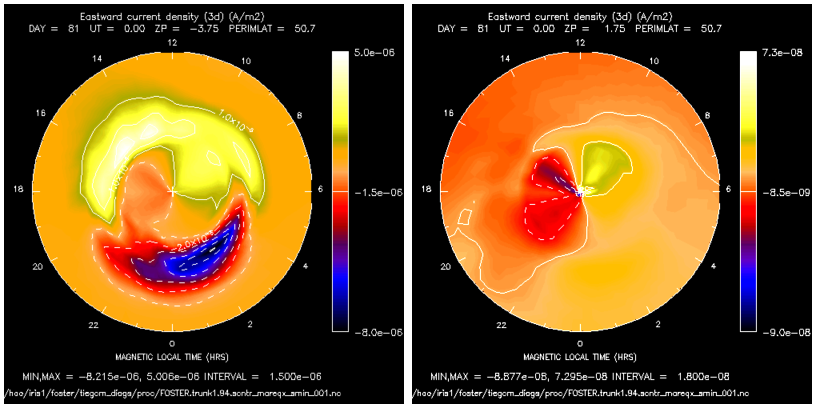
- JE13D
Diagnostic field: Eastward current density (A/m2) (3d on geomagnetic grid):
diags(n)%short_name = 'JE13D'
diags(n)%long_name  = 'Eastward current density (3d)'
diags(n)%units      = 'A/m2'
diags(n)%levels     = 'mlev'
diags(n)%caller     = 'current.F'
Je1/D is calculated in subroutine nosocrdens in source file current.F, and saved to secondary histories by subroutine mkdiag_JE13D (diags.F)
Note
JE13D is calculated and saved ONLY if the integer parameter icalkqlam is set to 1 in source file dynamo.F (the default is icalkqlam=0).
Sample images: JE13D North polar projection at Zp -4, +2
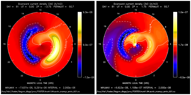
- JE23D
Diagnostic field: Downward current density (A/m2) (3d on geomagnetic grid):
diags(n)%short_name = 'JE23D'
diags(n)%long_name  = 'Downward current density (3d)'
diags(n)%units      = 'A/m2'
diags(n)%levels     = 'mlev'
diags(n)%caller     = 'current.F'
Je2/D is calculated in subroutine nosocrdens in source file current.F, and saved to secondary histories by subroutine mkdiag_JE23D (diags.F)
Note
JE23D is calculated and saved ONLY if the integer parameter icalkqlam is set to 1 in source file dynamo.F (the default is icalkqlam=0).
Sample images: JE23D North polar projection at Zp -4, +2
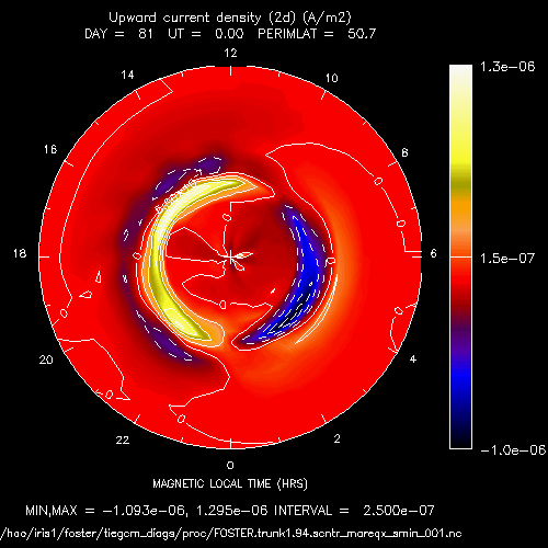
- JQR
Diagnostic field: Upward current density (A/m2) (2d mlat-mlon on geomagnetic grid):
diags(n)%short_name = 'JQR'
diags(n)%long_name  = 'Upward current density (2d)'
diags(n)%units      = 'A/m2'
diags(n)%levels     = 'none'
diags(n)%caller     = 'current.F'
Jqr is calculated in subroutine nosocrrt in source file current.F, and saved to secondary histories by subroutine mkdiag_JQR (diags.F)
Note
Jqr is calculated and saved ONLY if the integer parameter icalkqlam is set to 1 in source file dynamo.F (the default is icalkqlam=0).
Sample images: JQR North polar projection
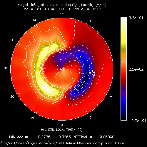
- KQLAM
Diagnostic field: Height-integrated current density (+north) (A/m2) (2d mlat-mlon on geomagnetic grid):
diags(n)%short_name = 'KQLAM'
diags(n)%long_name  = 'Height-integrated current density (+north)'
diags(n)%units      = 'A/m'
diags(n)%levels     = 'none'
diags(n)%caller     = 'current.F'
Kqlam is calculated in subroutine nosocrdens in source file current.F, and saved to secondary histories by subroutine mkdiag_KQLAM (diags.F)
Note
Kqlam is calculated and saved ONLY if the integer parameter icalkqlam is set to 1 in source file dynamo.F (the default is icalkqlam=0).
Sample images: KQLAM North polar projection
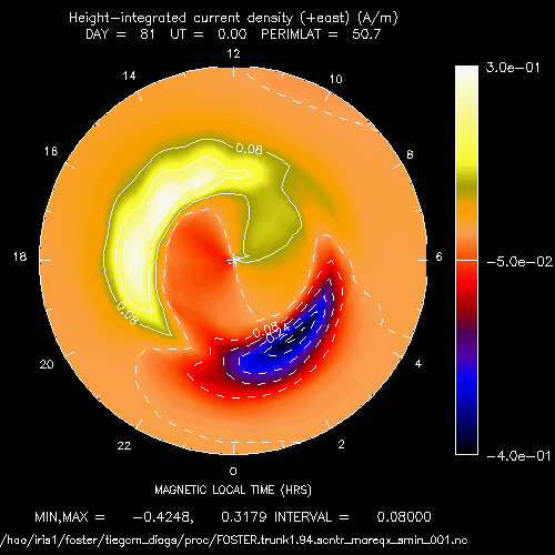
- KQPHI
Diagnostic field: Height-integrated current density (A/m2) (2d mlat-mlon on geomagnetic grid):
diags(n)%short_name = 'KQPHI'
diags(n)%long_name  = 'Height-integrated current density (+east)'
diags(n)%units      = 'A/m'
diags(n)%levels     = 'none'
diags(n)%caller     = 'current.F'
Kqphi is calculated in subroutine nosocrdens in source file current.F, and saved to secondary histories by subroutine mkdiag_KQLAM (diags.F)
Note
Kqphi is calculated and saved ONLY if the integer parameter icalkqlam is set to 1 in source file dynamo.F (the default is icalkqlam=0).
Sample images: KQPHI North polar projection