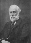
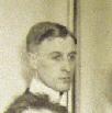
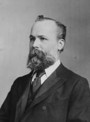
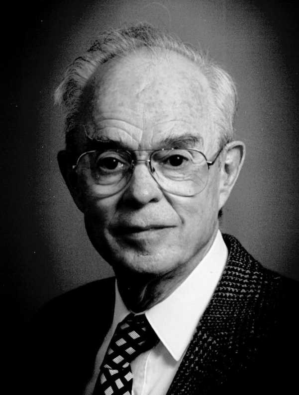
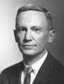
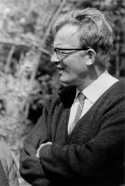
Professor C. A. Young, pioneer in astrophysics and especially solar physics. On the day he died there was a total eclipse of the sun.
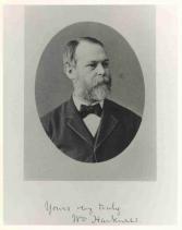
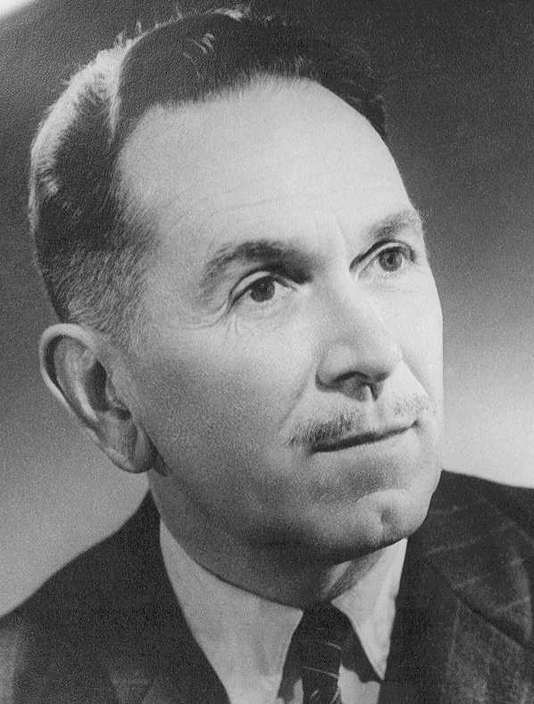
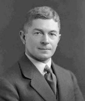
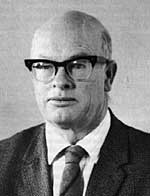
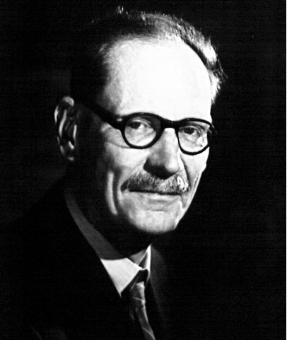
W. Harkness, civil war surgeon, astronomer, director of Naval Observatory, and, by his retirement, Rear Admiral.
P. G. Judge, HAO, NCAR, June 16 2011
Summary This web page recounts some of the more significant advances made towards the problem of understanding the mechanisms responsible for heating the sun's corona and driving the solar wind, problems first seriously recognized in the late 1930s and 1950s respectively.The document is written in several sections, each in historical order. By necessity the narrative makes no attempt to be complete, but instead attempts to highlight those efforts which led to particular insight into the problem of the generation, transport, and dissipation of mechanical energy from photosphere to corona.
SI units are used throughout.
The images and photographs used here are taken from sources freely available on the WWW.
| Professor C. A. Young, pioneer in astrophysics and especially solar physics. On the day he died there was a total eclipse of the sun. |
Until the 1930s, observations of the Sun's corona were only possible during total eclipses. At the eclipse of 1869, Charles Young and William Harkness independently observed a line in the green part of the spectrum, now known as the "green coronal line". These observations were made visually with spectroscopes. The line's origin was unknown and some believed it to belong to a new element, "coronium". There followed a period of 70 years of debate until it was finally identified by Edlén, along with several other lines of highly ionized complex atoms. | W. Harkness, civil war surgeon, astronomer, director of Naval Observatory, and, by his retirement, Rear Admiral. |
 P. Janssen, first director of Meudon Observatory, leader of many diverse scientific expeditions. |
The eclipse of 1871 was noteworthy because Pierre Janssen
observed Fraunhofer lines in the spectrum of the corona (presumably
the outer corona- later work by Grotrian
and others failing to find
such lines in the inner corona). When combined with earlier
polarization data, this demonstrated that the coronal spectrum is
formed in part by scattering of solar light, and is not a result of
diffraction, for example.
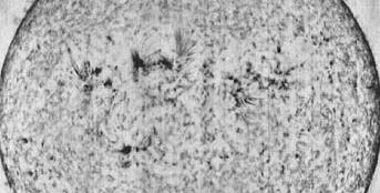
Beginning in the 1870s Janssen obtained photographs of photospheric granulation (Atlas de photographies solaires 1904) which were not bettered for 50 years, revealing a dynamic and turbulent surface. Such observations, albeit of the photosphere, are of direct relevance to coronal physics, the granulation being a source of mechanical energy for the overlying atmosphere. |
By 1878, eclipses had begun to reveal a
systematic relationship between coronal shape
and sunspot cycle, as noted by Ranyard in 1881 and Hansky in
1887. In 1871, the corona was roughly circular (maximum corona);
by the 1878 eclipse
streamers were dominant, and some resemblance of the corona to magnetic lines of
force was noted.
1908: Hale establishes existence of solar magnetic fields via the
Zeeman effect
 George Ellery Hale, pioneer in solar physics. |
In the article by Hale (1908),
"On the probable existence of a magnetic field in
sunspots", Hale invoked the Zeeman effect
to explain the doubling or splitting of certain spectral lines
observed for many decades in sunspots. Part of the inspiration was
his observation of helical gas motions around sunspots, suggesting to
him a magnetic origin or influence, reminiscent of
laboratory work involving magnetic fields.
While the magnetic fields were not measured within the corona, this discovery marks a critical moment for the corona in that much later work was to reveal the link between solar magnetism and the physics of the corona. In the following decade or so, Hale and his staff at Mt. Wilson established regularities in the magnetic properties of sunspots, including the polarity law which states that polarities of sunspot pairs reverse from one 11-year cycle to the next, and remain antisymmetric about the equatorial plane. He also established that the weak but measurable "global" magnetic field reverses every 11 years. |
W. Grotrian, Potsdam. |
In 1929 Walter Grotrian obtained spectra of the inner corona at
the eclipse that year. He found, instead of Fraunhofer lines, a broad
deficiency of emission in the violet part of the spectrum (Grotrian 1933).
In the 19th century, the absence of Fraunhofer lines caused some
confusion as to the origin of the corona (solar vs. lunar, for
example). By 1931, Grotrian suspected that the corona was anomalously
hot. If an earlier proposal by Karl Schwarzchild were correct, namely
that the coronal light originated by scattering of photospheric light,
then the strongest Fraunhofer lines should be visible, the weakest
being smeared by the Doppler motions even at temperatures as low as
5000K. Yet just a broad UV dip was observed. Perhaps the dip was
caused by scattering of Fraunhofer's strong H and K lines by electrons
at much higher temperatures. Grotrian (1934)
found the mean
speed of the scattering electrons to be consistent with a
Maxwellian of temperature around 350,000K.
In 1939, on the basis of new laboratory spectra in the vacuum UV obtained by Edlén, he proposed tentative identifications for the red coronal line with 9 times ionized iron, and a line at 789.2 nm with 10 times ionized iron (Grotrian 1939). While measurements were in the VUV, the wavelengths of such lines allowed the energy levels of the ground terms of the ions to be approximately calculated. From these, the wavelengths of the forbidden transitions could be estimated. This critical step was to inspire Edlén, Allen and others in the years to follow. |
 B. Lyot, who developed the coronagraph and birefringent filter, pioneer of coronal observations outside of eclipse. |
During the 1920s, Bernard Lyot tried to measure the polarization of
the planets, and
was led to try to observe Mercury in daylight. In the course of this
work, steps towards the development of the coronagraph were taken, and
Lyot detected Mercury only 1.5 degrees from the Sun.
In 1929, Barnard urged Lyot towards developing a coronagraph capable
of observing much dimmer objects, including the corona.
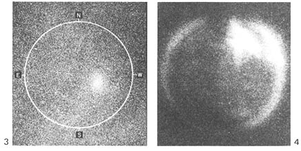
In 1930, equipped with Lyot's newly developed coronagraph, he & his team observed from Pic du Midi from July 25 to early August. These are the first credible observations of the corona outside of eclipse. (Several unconvincing claims were made by earlier observers.) He obtained the first photographs of the Green and Red coronal lines. In 1937, he suggested that the large apparent width of the green line might be due to thermal motions. By 1939, Lyot had found a total of 5 more unidentified lines, including infrared lines at 1074.6 and 1079.8 nm, and obtained spectral line profiles (Lyot 1939). |
| The coronal green line photographed by Lyot in 1930, using his coronagraph and spectrograph, outside of eclipse. From Lyot (1933). The abscissa is wavelength, the ordinate distance along a slit set tangentially to the solar limb. The line is the "fuzzy blob" between "E" and "South". The dark and bright horizontal lines are where the slit crossed the occulter (dark) and diffraction (bright). |
|
His work paved the way for the major advances made in the 1940s.
1943: Edlén's pivotal study of laboratory and solar spectra
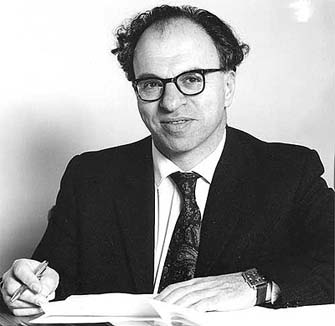
 Bengt Edlén, of Lund University. |
In 1943, in a famous paper marking perhaps the beginning of coronal physics, Edlén identified 4 of the known coronal lines against laboratory measurements obtained with a Siegbahn spectrograph and spark discharge, and many other observed lines using methods based upon atomic theory applied to the laboratory spectra (Edlén 1943). Edlén pioneered the powerful interpolation/ extrapolation spectroscopic techniques required for this work, melding observations with atomic theory. Interestingly, this paper is often mis-cited as being published in 1942. |
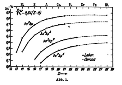
Edlén's figure 1, showing the variation of energy level parameters along isoelectronic series. Measurements from the laboratory follow the same smooth relationships with atomic number as the unidentified coronal lines, when formulated according to the theory of atomic spectra. |
All of Edlén's identifications were with ions which had between 9 and 14 electrons removed. The work was not readily accepted by the community, being published in the middle of WWII but also because of its important and far-reaching consequences. But with the work of Grotrian and Lyot, the evidence overwhelmingly pointed towards a corona containing distributions of electrons with energies sufficient to remove typically nine or more electrons from complex atoms.
Within a couple of years of this work, the corona was generally accepted as being extraordinarily hot. Edlén actually used an electron temperature near 250,000 K for calculations of electron impact excitation, noting that the the broad line widths and presence of a line of Fe XV suggest higher temperatures.
1948: Woolley & Allen's "well mixed" corona and revised radiation losses
 R. D. V. R. Woolley.
C. W. Allen |
Woolley & Allen (1948),
realized that the statistical balance between
the radiating ions of different charges is dominated by two-body
collisions, namely ionization and (radiative) recombination by
electron impact (along with, but independently from, contemporaries
Biermann and Miyamoto). The ionization equilibrium becomes
essentially just a function of electron temperature. This contrasts
with the local thermodynamic equilibrium approximation, in which
detailed balance between opposite processes must occur, for example
between three-body recombination and collisional ionization by
electron impact.
The electron temperatures found from these early calculations were a few million Kelvin. In addition Woolley & Allen's work marked an important conceptual change in the understanding of the corona. Previously, it had been accepted that elemental abundances are subject to large gravitational settling effects, because of the dominance of metal lines seen in the low chromospheric flash spectrum at eclipse, and the dominance of lines of the lighter H and He atoms in the higher chromosphere. By measuring the elemental abundances spectroscopically in the corona, with eclipse and coronagraphic data, it was clear that the corona is "well mixed". Heavy elements were therefore abundant in the corona, perhaps as abundant as in the lower atmosphere which was indeed mixed by convection. An important corollary is that coronal radiation losses, and estimates of the energy flux needed to balance them, had previously been underestimated by an order of magnitude or more, because losses from "metals" had not been considered. These estimates are given below. |
| Source | Flux density erg cm-2 s-1 | Luminosity erg s-1 | note |
| Allen (1973) | 6.27 1010 erg cm-2s-1 | 3.83 1033 erg s-1 | Total solar radiation | Biermann & ten Bruggencate (1947) | ≅ 103 | ≅ 6×1025 | protons & electrons | Woolley & Allen (1948) | ≅ 104 | ≅ 6×1026 | includes metals |
| Withbroe & Noyes (1977) | ≅ 1 × 10⁵ | ≅ 6×1027 | |
| | ≅ 2 × 10⁵ | ≅ 1028 | conductive losses |
| Withbroe (1988) | ≅ 8 × 10⁵ | ≅ 5 × 1028 | quiet Sun |
| ditto | ≅ 5 × 10⁵ | ≅ 3 × 1028 | coronal hole |
Withbroe & Noyes 1977 used direct measurements of UV, EUV and X-ray fluxes to estimate the radiation losses of the corona- by including the radiation losses from upper chromospheric and transition region material (including Ly-alpha) leads to a total radiative energy loss rate of ≅106 erg cm-2 s-1.
| Source | Flux density erg cm-2 s-1 | Luminosity erg s-1 | |
| Allen (1973) | 6.27 1010 erg cm-2s-1 | 3.83 1033 erg s-1 | Total solar radiation |
| Osterbrock 1961 | ≅ 3 × 10⁷ | ≅ 2 × 1030 | |
| Vernazza et al 1981 Table 29 | ≅ 4.6 × 10⁶ | ≅ 2.8 × 1029 | no Fe I/II |
| Anderson & Athay 1989 | ≅ 1.4 × 10⁷ | ≅ 1 × 1030 | Fe II dominant |
1964: Burgess' calculations of dielectronic recombination,
reconciliation of coronal temperatures
|
From
Edlen's (1943) work until 1964, many attempts were made to determine
the temperature of the ions and electrons in the corona, with
increasing levels of sophistication. The electron temperature enters
the emission line spectrum primarily by their effects on ionization
and recombination rate coefficients. The ion temperatures are seen
(as upper limits) in the widths of the emission lines (e.g., Evans
1963). Following a period of concern, in which the line widths gave
ion temperatures consistently lower than electron temperatures, the
two methods were reconciled finally by recognition of the importance
of "doubly excited states" accessible at coronal thermal energies,
which can auto-ionize or recombine in the electron-ion impact
dynamics. The influence of "dielectronic recombination" was thus
recognized as the missing ingredient by Burgess, following an earlier
suggestion by Unsold. (Burgess 1964, Burgess & Seaton 1964).
Although the new ionization equilibrium calculations including this process brought electron temperatures into better agreement with ion temperatures from line widths, at the same time, radio data were revealing electron temperatures lower by a factor of two or so (e.g., Kundu 1965). The radio data remain discrepant today (Noci 2003). This is perhaps not surprising, given the very different dependences of coronal line and radio continuum emission on electron temperature, density and the obvious inhomogeneity of the corona. |
 Kristian Birkeland. |
A clearer understanding of the origin of these terrestrial events came
with
Kristian
Birkeland: "From a physical point of view it is most
probable that solar rays are neither exclusively negative nor positive
rays, but of both kinds" - in other words a plasma.
This conclusion was driven in part by his
extensive knowledge of aurorae and laboratory work including the
famous experimental work on the terrella, in which cathode rays
were targeted at a magnetized sphere, producing aurora-like patterns
of light. This famous work is celebrated with images of Birkeland, the aurora and his terrella experiment on Norway's 200 Kr bank note.
|
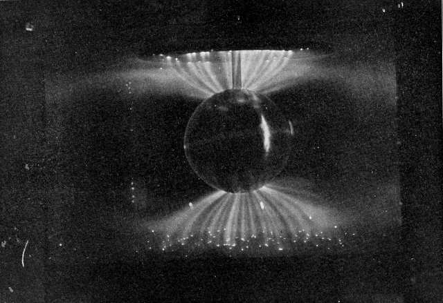 A Terrella photograph of cathode rays following magnetic field lines to the Anode (sphere), from charged plates. From "The Norwegian Aurora Polaris Expedition 1902-1903", by Birkeland. |
 E. W. Maunder |
Around the same time, Maunder (1904) quantified relationships known for some 50 years between sunspots, and geomagnetic activity. In particular, he was able to find a correlation between geomagnetic disturbances and the apparent solar rotation rate of 27 days, with an undeniably high significance. He concluded that "...our magnetic disturbances have their origin in the Sun. The solar action which gives rise to them does not act equally in all directions, but along narrow, well defined streams, not necessarily radial". Clearly, such actions were not consistent with a radiative origin. Such work was emphasized in subsequent decades, notably by Bartels (1932), who related these "actions" to streams of particles from "M regions" on the Sun. Bartels played a major role in the development of geomagnetism during the 20th century, both in Germany and the United States. Figure 7 from Bartels' review is included below. |
 Julius Bartels. |

 Ludwig Biermann, versatile theorist who predicted the existence of the solar wind. |
Comet tails were well known to exhibit evidence of forcing by the Sun (e.g., see Young 1896.) Yet the nature of the force remained unclear, until Biermann (1951) computed atomic parameters needed to estimate the radiation force on cometary molecular ions. He concluded that insufficient coupling of the radiation flux and the molecular ions existed to account for the observed behavior of comet tails. Instead, he estimated that charged particles flowing from the Sun, suspected of being the cause of geomagnetic phenomena for almost a century, with speeds of several hundred km/sec and densities of 100-1000 particles per cm3 could account for properties of comet ion tails. Thus, in 1951 he surmised that the Sun must emit corpuscles- there was indeed a "solar wind". |
 Sydney Chapman (1888-1970) made major contributions to geomagnetism, stellar dynamics, meteorology and the kinetic theory of gases and plasmas. |
The next part of the story unravels quickly, beginning in 1957 when
Sydney Chapman
showed theoretically that coronal material
near temperatures of 1MK must be very efficient conductor of heat- the
corona would be hot over a considerable fraction of the inner solar system.
Using this result, Parker (1958a) examined the force and thermal balance of coronal matter. He showed that a corona in hydrostatic equilibrium exerts a finite pressure at infinity, which could not be balanced by the known pressures in the interstellar medium. Parker therefore concluded that the corona must inevitably expand according to the hydrodynamic equations. Realizing that this flow represents a very significant sink of energy, namely 3x1028 erg/sec, in addition to the 1027 erg/sec estimated then (modern values are larger) to allow for losses from the static corona due to radiation and conduction, Parker (1958b) showed that hydromagnetic waves may be responsible for supplying the expanding corona with sufficient energy. |
 E. N. Parker, cosmic electrodynamicist, first winner of the Hale Prize, winner of the Kyoto Prize awarded for a lifetime achievement in basic science, among other awards. |
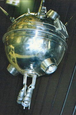 Luna 1. Luna 1.
|
Then, in January of 1959, direct measurements of particles coming from the Sun were made with the Soviet spacecraft Luna 1, as it emerged from the protection of the earth's magnetic shield into interplanetary space. The plasma measurements broadly confirmed Biermann and Parker's work, were reproduced by the Luna 2 spacecraft launched in September 1959. However, the direction of the flowing ions was not determined until American spacecraft flew into the solar wind. In 1962, Mariner 2, on its way to Venus, sampled the solar wind along its trajectory. (Earlier suggestive work using Explorer 10 had not convincingly left the earth's magnetic influence.) The wind was found to flow continuously, but with large fluctuations. |
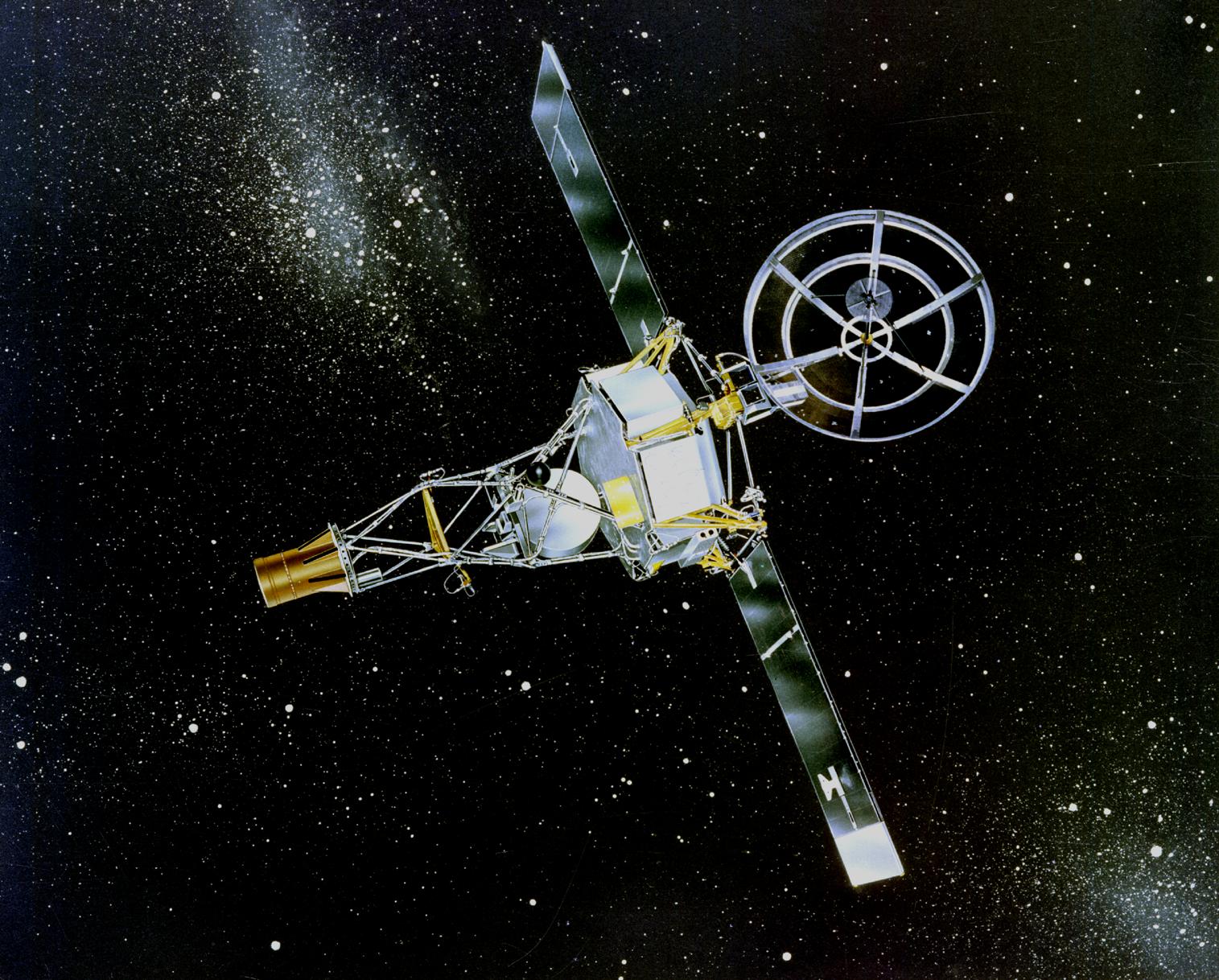 Mariner 2 (artistic rendering). Mariner 2 (artistic rendering).
|
A major step was taken with the discovery of "coronal holes" from EUV disk observations from OSO-6 (Withbroe et al. 1971). During the SKYLAB era, sufficient data were acquired to prove that the coronal holes were related to the streams from Bartels' "M regions" on the Sun, nicely tying together the less direct but statistically significant work begun by Maunder and others (Jordan 1974, Neupert & Pizzo 1974). Now it is known from spacecraft measurements that the solar wind has essentially two characters, "fast" and "slow". Coronal holes are sources for the "fast" solar wind.
The work of Parker (1958a, 1958b) remains a landmark, being the first to recognize and deal with the physics of the solar wind / solar corona as one system.
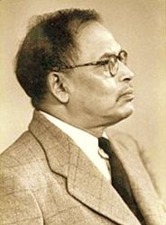 Meghnad Saha, of "ionization equilibrium equation" fame, also proposed a theory of coronal emission lines based upon fission of actinide elements (e.g., 235U). | Meghnad Saha proposed that the high ionization states of
ions seen in solar corona might find their origin in nuclear
processes. Specifically, in Saha 1942 and
Saha 1945
he proposed that fission of
235U, 238U, 232Th and
229Pa followed by the impact of the fission products on the
ambient atmospheric particles might lead to the observed emission of ions of
iron, for example.
The main argument against this picture, (with others outlined by Saha himself in the 1945 paper), are that the fission products for nuclear binary, tertiary or quaternary processes are expected to have particle kinetic energies of order 102 MeV. For an iron nucleus the speed expected is thus of order 0.05c or 2x10⁴ km/sec, some 3 orders of magnitude larger than observations indicate (e.g., Lyot 1939). Saha also argued against the interpretation of coronal emission lines in terms of the impact of meteoric material, originally proposed by Vand (1943). Saha's contention was that to strip 10 or more electrons from meteoric atoms would only occur in much deeper layers of the Sun, and also that line width observations by Lyot were incompatible with these ideas. It is interesting that Saha did not appear to realize that the measured line widths were also incompatible with his fission proposal. |
|
Ludwig Biermann. | In 1946 and 1948, Ludwig Biermann examined the proposition that acoustic disturbances generated by granular motions 400 km below the solar surface can propagate and dissipate in the upper photosphere and lower chromosphere. He was seeking to understand the observed "turbulence" in the chromosphere and the radiation emitted from it. His work recognized that only waves above the acoustic cutoff frequency (a natural frequency of the stratified atmosphere, it corresponds to a wave period of 3 minutes) could propagate upwards. He estimated that the dissipation in the upper photosphere and chromosphere, via radiation losses of the material compressed by the waves, would yield energy insufficient to heat the corona. |
 Martin Schwarzschild, who proved that granulation is convection from high altitude observations. He made major contributions to stellar structure and evolution. |
Independently, in 1948, Martin Schwarzschild estimated
the noise arising from solar granulation, and its
ability to heat the corona (Schwarzschild 1948). From measured
properties of the granulation he estimated the energy flux of noise
(acoustic waves) with the energy requirements of the corona. His
paper states clearly the nature of the coronal heating problem
(compare this with Alfvén's picture below):
"The mechanism which maintains the high temperature of the corona has to fulfill two conditions: first it has to provide energy at a rate equal to that of the heat loss of the corona, and, second, it has to provide the energy in such a form that it can be delivered to the material of the corona at its high temperature." Schwarzschild adopted the coronal energy flux estimate of 103 erg cm-2 s-1 from Biermann and ten Bruggencate from 1947. This which was soon found to be much too small (Woolley & Allen's 1948 work), because the corona corona was erroneously assumed to be gravitationally settled, such that only hydrogen, helium and electrons would be present in the corona. Schwarzschild assumed that dissipation of wave energy sets in when the wave amplitude approaches the sound speed, (hence leading to non-linearities, i.e. shock waves), which he estimated to occur 800 km above the top of granulation. He implicitly assumed that a a sufficiently large fraction of the wave energy survives the chromosphere to be able to reach the corona. |
 Évry Schatzman, who developed a complete shock wave theory of the solar corona. | An important step was taken in 1949 by Évry Schatzman, who treated explicitly the steepening of linear waves into shocks. Applying the shock wave theory of Brinkley and Kirkwood, simplified to the limiting case of weak shocks, and using a principle of invariance, he developed a model of the chromosphere/corona which included the effects of wave refraction, heat conduction and radiation in bound-free and free-free transitions. This work represents the first physically "complete" model in the sense that the energy equation was solved, balancing heat gains from the shocks with losses due to conduction and radiation. |
However, later work revealed some details of Schatzman's model
as problematic- the neglect of (dominant) bound-bound radiative
transitions and the attempt to fit all off-limb data simultaneously in
an inhomogeneous thermal environment being serious issues, leading to
shallow temperature gradients at odds with later UV and EUV disk data.
Like Schwarzschild, Schatzman used a value for the energy
requirements of the quiet corona near to 103
erg cm-2 s-1 from Biermann and
ten Bruggencate (1947), now known to be 2-3 orders of
magnitude too small because of the neglect of bound-bound transitions
in "metals" which would be present in a well mixed, not fractionated,
corona
(Woolley & Allen 1948). Thus acoustic waves are no longer considered as
viable candidates for coronal heating (see "The failure of acoustic waves"
) below.
Giovanelli 1946-1949: Discharge of electrical currents
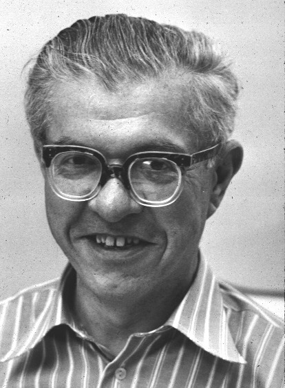
 R. Giovanelli, solar observer, theorist, and originator of critical ideas behind "magnetic reconnection". |
Between 1946 and 1949, Giovanelli developed a theory by which magnetic energy associated with sunspots can be converted to particle acceleration. In his original picture, electric fields induced by the evolution of sunspot magnetic fields (Faraday's Law) are generated which accelerate particles, leading to electrical currents. Resistive dissipation of the currents (collisions of electrons with hydrogen atoms and ions) then heats chromospheric plasma, leading to flares. This process is an electrical discharge. A critical aspect of Giovanelli's work which survives today is the importance of magnetic neutral points (zero magnetic fields) within the atmospheres expected above many different sunspot types. Neutral points are places where such acceleration can occur - elsewhere electrons are confined to follow magnetic field lines B so that induced electric fields (v x B) cannot accelerate the plasma. Giovanelli's work thus introduced the idea of changing the topology of the magnetic field, an important concept for coronal heating. Modern theories of reconnection share this property in spite of the fact that the arguments used by Giovanelli to evaluate the electric fields are untenable (see the arguments by Piddington and Cowling). The MHD system generally evolves slowly, because of the huge inductance, to generate motions (Alfvén waves) in the fluid and not electrical discharges. Any field-aligned electric currents in the frame of motion of the fluid are essentially zero because of the high conductivity. |
Herman Bondi. |
In a paper entitled "On the structure of the solar corona and chromosphere", the authors attempted to explain the existence of the chromosphere and corona in terms of the accretion of interstellar material. The thermal energy is supplied by accretion of interstellar material, drawing energy from the gravitational potential energy of circumsolar material. (In 1943, Vand had made a similar proposal based upon the accretion of interplanetary material, see Vand 1943). |
Fred Hoyle. |
This theory was later discredited upon several grounds, observational and theoretical (e.g., Shklovskii 1961, pp. 383-386.) The later discovery of the solar wind, for example, is not compatible with the accretion hypothesis for the Sun. As Shklovskii pointed out, the source for the mass, momentum and energy of the corona is the Sun itself.
 Hannes Alfvén, Nobel Laureate in Physics (1970), originator of many ideas in MHD. |
In the context of the relatively new subject of
magnetohydrodynamics (MHD) - essentially invented by Alfvén himself -
Alfvén proposed that waves generated in a highly conducting,
magnetized fluid may propagate and eventually dissipate in the
corona. The turbulent and dynamic nature of granulation in the solar
surface was known since Janssen's work in the 1870s, and magnetic
fields were
known to exist at
the Sun's surface since the work of Hale in the 1900s. Furthermore,
the corona itself was noted to have appeared to have structure
reminiscent of magnetic lines of force seen in the laboratory and
around the earth already by Bigelow in 1899.
The waves he considered were those he discovered theoretically and called "magnetohydrodynamic" waves in 1942-3, namely transverse oscillations which are not compressible- the "Alfvén waves" (Alfvén 1943). |
In his important 1947 paper, granular motions were assumed to generate fluctuations in the magnetic fields. Based upon solar properties then known, Alfvén estimated the generation, reflection and dissipation of his "magnetohydrodynamic" (now known as "Alfvén" waves), to arrive at a plausible model for explaining the temperature and energy requirements of the corona. He assumed the magnetic field to be primarily the global (dipole-like) component identified by Hale and colleagues. Waves with frequencies above those reflected by density gradients (those with λ / scale height < 4π) propagate into the corona where the finite conductivity leads to Joule dissipation and coronal heating. Alfvén invoked Cowling's (1945) "transverse conductivity" to provide sufficient dissipation. Later, Cowling (1953) showed that Alfvén had not applied the correct form of the conductivity to the case of fully ionized gases, and had over-estimated the Joule dissipation enormously. The work of van de Hulst (1951) was nearer the mark, showing that dissipation of Alfvén waves was weak and dominated by viscous dissipation in the Sun's atmosphere.
Although the magnetic and thermal structure
of the solar atmosphere, wave generation efficiency, and electrical
conductivities used were later shown to be inappropriate, this
paper must nevertheless be considered a major landmark in that it contains
many essential ideas which have dominated the subsequent
literature concerning coronal heating:
Alfvén makes two further observations of importance: First he points out that the accretion proposals for coronal heating could not explain the coronal variations with the magnetic activity cycle. Second, he ends with an estimate of the coronal temperature near 2 million K, very close to currently accepted values. (This was derived from the radial brightness variations of the corona with the assumption that the corona is supported against gravity by an outward-directed hydrostatic temperature gradient.)
For completeness it is worth noting that compressibility was first treated in the linearized MHD equations of motion by Alfvén's colleagues Åström and Herlofson in 1950, leading to the two magneto-acoustic modes. The incompressible Alfvén waves were first detected in the laboratory by Lundquist (1949).
Although much later, Warwick made a suggestion which deserves a mention amongst "initial proposals" for atmospheric heating, in the context of mechanisms for flares. Warwick (1962) examined the idea that energetic particles might be generated in (sub)-photospheric layers which, although of little significance to the energy within such deep layers, might nevertheless be of vital importance in the overlying chromosphere and corona, where most of the flaring plasma resides. He argued that protons of 100MeV (known at the time to be associated with flares) might emerge from as deep as 400 km from beneath the photosphere into the chromosphere and corona. Subsequent interactions with the atmosphere are then supposed to lead to flare emission and high energy proton escape. This work is thus related to the proposal by Saha (1945).
Several problems exist for this picture. Firstly, no explanation for the rapid onset of flares exists. Second, the Fermi process requires a collisionless environment, thus there is no way to reach the high energies needed for escape from the much lower energy thermal pool of available protons in the photosphere. Thus, while Warwick correctly pointed out that the energy needed to drive flares can be found in the dense photosphere, there is no viable mechanism by which these layers can generate very high energy particles extending into the corona.
Later, Athay & White (1978, 1979) showed from observations of emission line profiles from the OSO-8 spacecraft, with models of chromospheric lines, that acoustic waves carry an energy flux insufficient to heat the upper chromosphere and corona. The main differences between their work and the efforts in the 1940s are twofold:
Sometimes one reads that this work discounts the possibility that
Alfvén and fast mode waves cannot provide the necessary
energy. However, this assumes that the
Alfvén speed VA does not exceed the sound speed in
the upper chromosphere.
It has yet to be demonstrated through measurements that this is the
case. Simple estimates suggest indeed that VA >
C
The 1970s also revealed other problems with models based only on acoustic waves. Fully consistent static models could not be constructed because the wave pressures needed to carry the energy were several times larger than the total weight of overlying coronal material (McWhirter et al. 1975.)
 Henk van de Hulst, photo by Rob Rutten. |
In 1949-1950, van de Hulst (1951) linearized the MHD equation of motion including finite conductivities and viscosities, with Maxwell's equations. Background plasma and magnetic conditions were assumed to be homogeneous. van de Hulst credits Herlofson's (1950) publication as the first to identify the two magneto-acoustic waves, but of course these also dropped out of van de Hulst's analysis in the limits of small v/c and zero conductivity and viscosity. He appears to be the first to coin the terms "slow" and "fast" for the magnetoacoustic modes. The novel aspect of this work is the inclusion of viscosity and the realization that it is far more efficient than resistivity at removing energy from Alfvén waves both in the interstellar medium and in the Sun's atmosphere (he actually considered the chromosphere). Unlike Alfvén (1947), he used scalar transport coefficients then available, which turn out to be more appropriate in the fully ionized corona plasma (Cowling (1953). Using van de Hulst's results with modern transport coefficients, viscous damping lengths (1/e) are of order 100 solar radii for an Alfvén wave with 5 minute period, scaling with (period)2. (5 minutes was chosen here from the time scale of evolution of granulation, and the prominent frequency seen in the global oscillation modes at the surface). For Joule dissipation, damping lengths are many orders of magnitude larger. Thus, the energy in such waves propagates almost without attenuation by these processes in the corona, at least in models which have nearly homogeneous plasmas. It is thus very difficult to heat the corona with such waves.
|
 T. G. Cowling.
J. H. Piddington
| In independent articles published in 1953,
Cowling (1953)
and Piddington (1953)
examined earlier work (including that of Giovanelli) on the generation of electric
fields in plasmas in motion. They conclude that the mis-application of
Faraday's law (the equation of electromagnetic induction) has some
problems. For example, Cowling says that it "...is responsible for the failure of many electromagnetic theories of solar phenomena. The induction is essentially an inertia effect; induced currents flow in such a way as to oppose the motions and changes of field to which they are due. The inertia effects are enormous in a large conductor like the sun; hence a favorable cause may be wholly unable to produce a desired effect in the relatively short time which is permitted." In the language of electric circuits, the plasma's inductance L is extremely high because of the large physical scales. Coupled with the low electrical resistance R of ionized plasma (similar to metallic copper), the time for the development of the induced electric field in the circuit, L/R, is enormous. Piddington focussed upon the mechanical back-reaction of the Lorentz force, through a careful study of the conductivity tensor and associated currents. More specifically, he examined Giovanelli's flare theory, prominence models, models of cosmic ray acceleration and solar radio emission. He argued that models for acceleration of particles due to electric fields along the magnetic field (as proposed by Giovanelli) are untenable. |
Cowling further argued that MHD requires one to evaluate the current density from curl B and use the conductivity tensor to evaluate the electric field and (if needed) the resistive dissipation of electromagnetic energy. Giovanelli instead adopted Faraday's law from the outset. The difference is that force balance is set by the Lorentz force (curl B) x B on a time scale determined by the Alfvén speed and the plasma dimensions. This time scale is far shorter than the inductive time scale. Thus the force balance fixes B, and the current density curl B, from which the instantaneous electric field can be reliably evaluated using Ohm's law (itself from the kinetic equation of motion for electrons).
Cowling also realized that Alfvén's proposal for heating by MHD waves presented difficulties. He argued that the use of his transverse resistivity (Cowling 1945) by Alfvén was incorrect: for ionized plasma the wave motions involved do not increase particle collisions so that the resistivity is unaffected. (Cowling's transverse resistivity is appropriate when wave motions affect different plasma particles differently, creating "friction", such as occurs when magnetic waves propagate through a partially, not fully, ionized fluid.)
These basic difficulties remain today. Cowling and Piddington's insights have focused attention of on these essential problems, and has shaped the later research on coronal heating.
One important development was made when Dungey (1958) clarified and corrected Cowling's statement that "... The induction is essentially an inertia effect; induced currents flow in such a way as to oppose the motions and changes of field to which they are due." Near a neutral point, Dungey (1953) had demonstrated that, under the action solely of the Lorentz force, the current tends to become enhanced. In this configuration, therefore, locally Lenz's law is reversed in that the changes amplify those responsible for the initial perturbation. Dungey (1958) also argued (but did not prove) that pressure gradients were unlikely to be able to halt the tendency for this instability to arise. Sweet's (1958) report at the same meeting and Parker's work (see below) suggested that Dungey was correct, the instability would proceed until the energy of inflow balanced heat losses due to finite conductivity.
The viewpoints of Cowling and Piddington have recently been re-iterated by Parker (2007). Parker argues that great danger awaits those applying electrical circuit analogs to MHD systems: in MHD, changes in the system (for example at the system's boundaries) occur via the interaction between the plasma and the magnetic field, according to the equations of Newton, Maxwell, Boltzmann and Lorentz. Electric currents and electric fields adjust themselves accordingly, playing only a minor role in the large-scale dynamics. Thus he argues that the correct paradigm for understanding MHD systems is to focus first upon the velocity and magnetic field to determine the dynamics (v,B paradigm), from which the electrical currents and electric fields can be derived, if needed, for example to examine Joule heating (j,E paradigm ).
Thus, in his chapter 11, Parker gives an explicit example of the dynamics of an MHD system (a twisted flux tube embedded in an uniform, unmagnetized medium) responding to the sudden blockage of the associated electrical currents. In the "electrical circuit" picture, a large EMF is set up which some authors claimed is capable of accelerating charged particles to high energies. But the physics of the MHD system must take into account the coupling between the fluid and magnetic fields according to the laws of Newton and Maxwell. In reality then, the system evolves dynamically so as to keep the electric field in the frame of the moving plasma zero: no discharge is possible because the energy associated with the electrical current is therefore channeled into MHD motions- in this case torsional Alfvén waves. No explosive behavior occurs and no energetic particles result. Theories based upon simple electrical discharges, for example in the double layer theory of flares by Alfvén & Carlqvist (1967) are thus untenable.
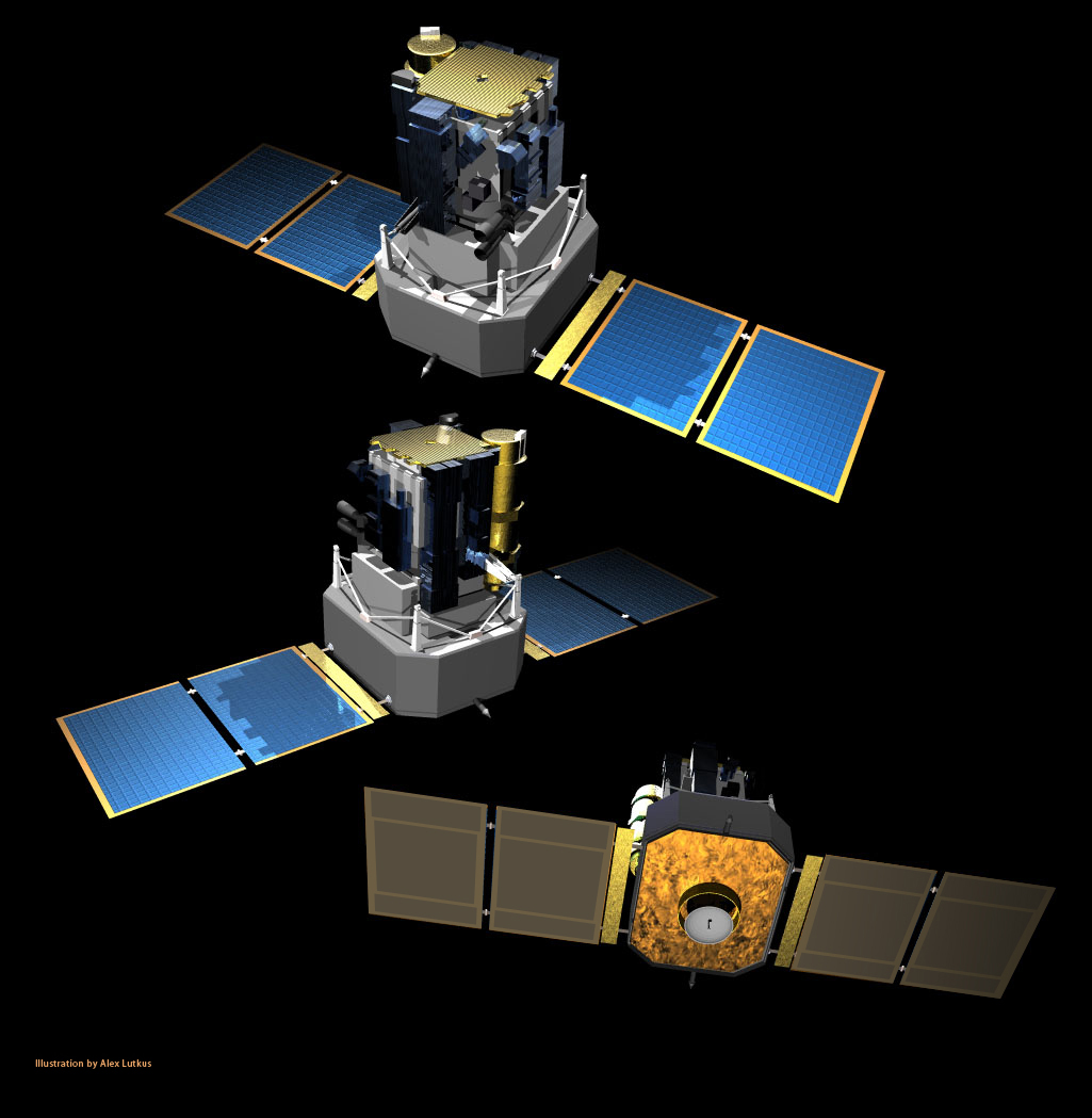
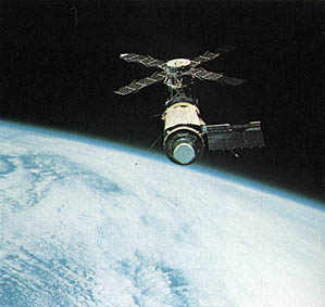 SKYLAB in orbit, 1973 | SKYLAB was
the first manned orbiting observatory. Eight instruments were mounted
on SKYLAB's Apollo Telescope Mount (ATM), which built upon the successful
series of Orbiting Solar Observatory spacecraft (OSO)
as well as sub-orbital rocket flights. ATM
is seen in the picture with solar power arrays attached, on top of the
main module.
Three X-ray
instruments were part of the ATM (S-020, S-054, S-056), a UV slit
spectrograph (S-082B), a UV slitless spectrograph (S-082A) and a
scanning spectral imager (S-055). A coronagraph (S-052) and two
Hα telescopes were included.
SKYLAB's impact on our understanding of the solar corona and the controlling magnetic fields is difficult to overestimate: "Especially illuminating has been the recognition of the extent to which the Sun's magnetic field is responsible for the structure, dynamics, and heating of the Sun's outer layers." -- Leo Goldberg, then of Kitt Peak National Observatory, from the foreword in the monograph A New Sun: The Solar Results from Skylab by J. Eddy.
|
|
Pre- SKYLAB X-ray images of the Sun obtained using sub-orbital imagers between 1963 and 1969. These few snapshots can be compared with the many months of almost continuous data from SKYLAB. From A New Sun: The Solar Results from Skylab.
|
SKYLAB's primary contributions to our understanding of the
corona are
|
 In these SKYLAB data, bright points are seen at the base of coronal plumes, the latter having been observed at eclipses since the 19th century.
|
Simultaneous images in an upper transition region emission line (left) and of a coronal line (right) from S-082A on SKYLAB. Taken from A New Sun: The Solar Results from Skylab. The loops in the active corona have counterparts near the footpoints in the upper transition region. Notice the chromospheric network in the latter image.
|
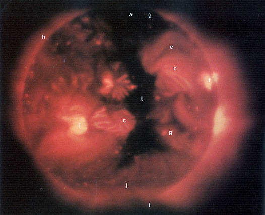
The whole corona seen in X-rays with SKYLAB, showing plasma near 2 MK. Bright points (g), active region loops (c,f), loops connecting different active regions (d) and a large coronal hole (b) are visible. Magnetic fields organize all the structure in this picture. From A New Sun: The Solar Results from Skylab.
|
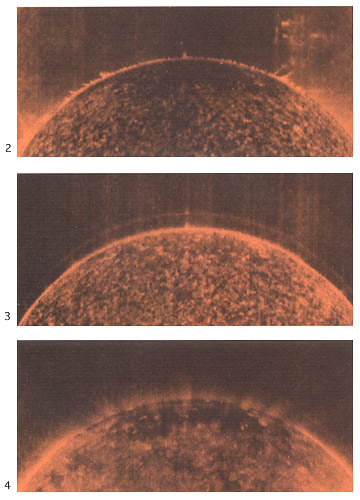
|
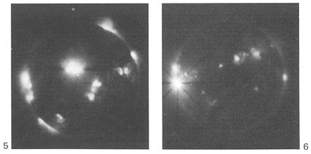
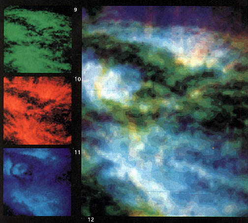
These SKYLAB images are of the low chromosphere (9), colored green; transition region (10), red; and the corona (11), blue. In the larger photo (12) the three pictures and colors are added together to form a 3-color image. These active region loops are too hot to be visible at chromospheric temperatures and too cool to show up sharply in the corona, where we see only the diffuse envelope of their outer sheaths. Loop structures are most clearly seen at temperatures in the transition region near 450 000 K (10). From A New Sun: The Solar Results from Skylab.
|
|
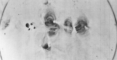
|
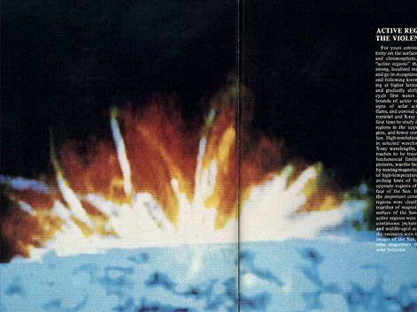
Active regions seen at the limb in a 3 color image (blue=chromosphere, red=upper transition region, green=corona). Active regions are defined by soaring magnetic fields; they consist of hot loops of high-temperature gas, trapped and contained by arching lines of force whose footpoints stand in opposite regions of high magnetic field on the surface of the Sun. Magnetic loops in new, old, and middle-aged active regions account for most of the emission seen in SKYLAB'S ultraviolet and X-ray images of the Sun. From A New Sun: The Solar Results from Skylab.
|
|
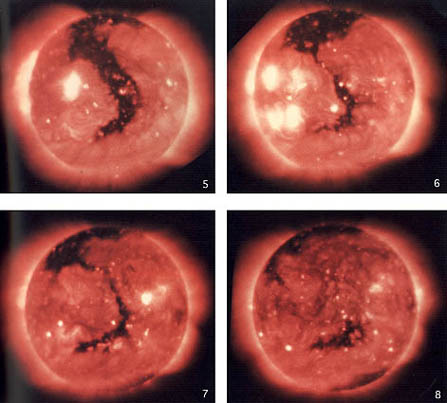
Evolution of a coronal hole over about 3 months is shown in soft
X-ray pictures taken at spacings of one solar rotation-about 27
days apart. Curiously, coronal holes rotate as though
attached to a solid Sun, unlike the slipping layers of the photosphere
and chromosphere, which rotate much faster at the equator than at the
poles.
From A New Sun: The
Solar Results from Skylab.
|
|
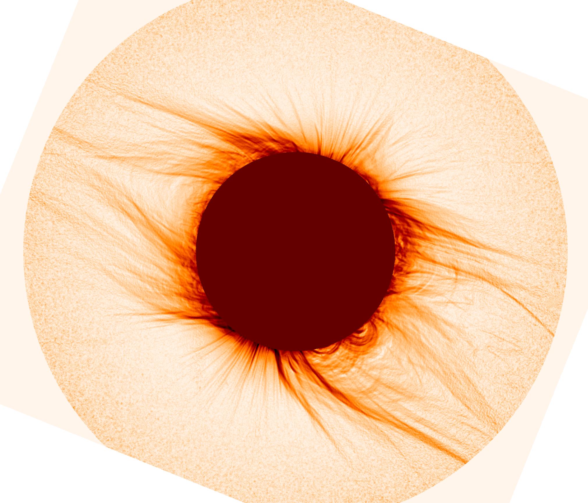
 A white-light image of the eclipse of July 11 1991 obtained by the High Altitude Observatory and Rhodes College. A "Newkirk Camera" was used which has a radial density filter to try to make coronal structures equally bright at different radii. |
All EUV and X-ray images from SKYLAB reveal those regions where the temperature is suitable for a certain transition to emit. Furthermore, the intensity is almost always proportional to (density)2, integrated along a given line-of-sight. EUV and X-ray emission from particular ions in the corona therefore provides a highly special, filtered view of the corona. White light images, formed by electron scattered photospheric light, have essentially no dependence on the electron temperature and the intensity is proportional to the line-of-sight integral of the density along the line of sight. White light images (obtained during eclipse or from polarized brightness images obtained from coronagraphs) therefore present us with a less special, complementary view of the corona. |
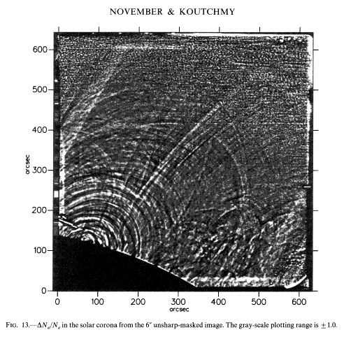
The highest angular resolution data yet obtained for the corona were acquired with the 3.6m CFHT telescope which happened to lie in the path of the total eclipse of July 11, 1991. The Sun was relatively active. The data, acquired quickly (up to 30 frames per second) revealed (November & Koutchmy 1996)
|
Figure 13 from November & Koutchmy (1996). The figure displays ΔNe/Ne, the departures of the electron density from a local mean, along a line-of-sight intercepting the SW (lower right) quadrant of the image above. The gray scale varies from zero to 2.
|
The relatively uniform density derived from these data stands in contrast to the appearance of the extremely inhomogeneous EUV/X ray corona. But the white light data should be trusted more because they directly reflect the density structure of the corona. This point is re-inforced by photometric-quality white light data from the 1998 February 28 eclipse:
Data from HAO's POISE instrument deployed in Curacao in February 1998. The left panel shows the Newkirk Camera image, the right a numerically enhanced version of the image. EUV data more closely resemble the enhanced image. The white light data show that, at the instrumental resolution, the Sun's coronal density is more homogeneous than the dramatic EUV/X ray images suggest.
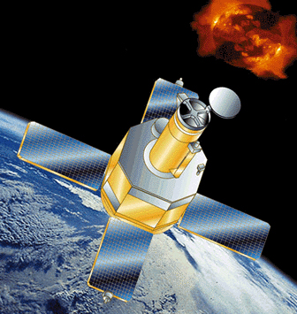
 Artist's illustrations of SOHO. | The Solar and Heliospheric Observatory
(SOHO)
is a joint NASA/ESA spacecraft
which sits between the earth and the Sun, designed to provide an uninterrupted
view of the Sun and measurements of the solar wind.
SOHO's impact on our understanding of the solar corona and the controlling magnetic fields is profound:
|
 Artist's illustration of TRACE in orbit. | TRACE was the first US
mission to have a completely open data policy. The mission consists of
a multi-layer telescope
designed to take correlated images in a range of wavelengths from
the visible to the EUV. The
different wavelength passbands correspond to plasma emission
temperatures from photospheric temperatures 4,000,000 K.
TRACE has provided the highest resolution images of the corona to date. It's impact on our understanding of the solar corona and the controlling magnetic fields is profound:
|
The time needed for diffusive annihilation of magnetic fields in a volume of characteristic scale L containing continuous magnetic fields on the same physical scale, is
where η is the magnetic diffusivity (η-1= σμ0, σ is the plasma conductivity and μ0 the permeability of free space). In terms of the magnetic Reynolds number (Lundquist number) RM=LVA/η, with VA the Alfvén speed,
L/VA is the time scale for propagation of MHD waves- the dynamical time scale for the magnetic fields, of order 1-10 seconds in the corona over a sunspot. Now RM is of order 3×10¹⁴ in the corona over sunspots, so that the diffusive time scale is of order 3×10⁶ years.
Now, solar flares were known to release energy on time scales of an hour or less. It had been recognized that both the particle acceleration and energy released by solar flares had to have its origin in the magnetic fields overlying sunspots (e.g., Giovanelli, Parker 1957b). there being no credible alternatives.
Thus, much early effort focused on trying to see how the time scale for magnetic field annihilation might be reduced by many orders of magnitude, the flare phenomenon representing perhaps the most extreme form of a coronal heating mechanism.
Dungey 1953: Discharge of electrical currents, revisited
|
In 1953, Cowling had pointed out that thin current sheets (of
thickness of a few meters) would be needed to explain solar flares via
Joule dissipation in an electrical discharge. Dungey (1953) showed that discharges are
unlikely to occur anywhere except at neutral points. He also argued
that thin sheets may indeed form owing to the collapse of magnetic
fields near an "x-type" neutral point. The collapse arises because the
configuration is unstable due to the action of the Lorentz force
induced by the currents on the plasma, providing the external boundary
conditions permit the evolution to occur. This is an ideal MHD
instability. The growth time is on the order of
L/VA.
He argued that under conditions of large but finite conductivity,
within the very narrow current sheets,
"the lines of force... can be broken and
rejoined there".
This is probably the first explicit statement of the concept of field
line breaking followed by
reconnection.
He visualized the X-type reconnection as the decay of the toroidal component of the magnetic field associated with the resistive decay of the electrical current induced at the X-point, as follows: |
 J. W. Dungey, pioneer in the physics of reconnection, especially its application to the earth's magnetosphere and geomagnetic storms. |
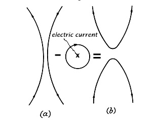
Dungey's figure 2 (adapted to highlight the decaying field [circular loop] associated with the induced electric current). The toroidal field associated with the current flowing into the screen/page is shown (circular field line). X-point reconnection can be envisaged as the decay of this field component (represented by the minus sign in the figure), leading configuration (a) to evolve into configuration (b). (b) appears to be just a rotated form of (a), but the stronger magnetic tension forces in (b) tend to separate the field lines leading to a different configuration unlikely to reconnect further.
In this way it is clear that the X configuration must evolve to the lower-energy, disconnected state of two "U"-shaped field lines seen in the figure.
A complete mathematical model for a particular magneto-fluid configuration was built by Chapman and Kendall (1963), showing that Dungey's ideas, based upon physical arguments and simplified (force-free) mathematical models, were well founded.
Dungey's work is significant because it began the study of the role of current sheets in the dissipation of magnetic fields in highly conducting plasmas.
In an effort to quantify these ideas, specifically to see if flare time scales might be accounted for by the formation and decay of current sheets, in 1956, Sweet (reported in Sweet 1958) studied magnetic fields explicitly including resistivity and gas pressure effects near a neutral point in the corona. The bipolar fields of two sunspots were brought into contact in the corona. Sweet found that conditions far from the neutral point were important to the expected dynamics, and concluded that owing to Joule dissipation, the configuration indeed can lose equilibrium via formation of a thin current sheet (the "X" point evolving into to "Y" points connected by the sheet), through which plasma and magnetic fields flow. The accompanying reconnection occurs on a time scale much faster than the diffusive time scale of the whole system. Parker studied Sweet's problem immediately following Sweet's talk, within the framework of MHD, publishing his results in 1957 (Parker 1957a).
 P. A. Sweet, pioneer in stellar interior and magnetized plasma studies.
E. N. Parker. |
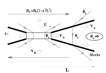
Parker applied a boundary layer treatment to the simplest case- that of oppositely directed magnetic fields brought together at a neutral line (or sheet, in 3D), in a steady state, with geometry shown below (adapted for SI units from Kulsrud 2000):
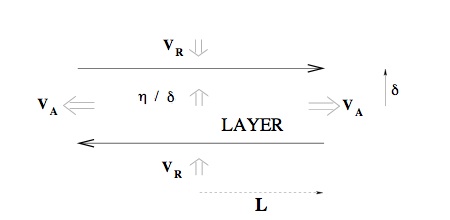
The Sweet-Parker diffusion layer. In a steady state the magnetic diffusion speed η/δ balances the incoming reconnection speed VR, and the inflowing volume 4VRL balances the outgoing volume 4VAδ (the plasma is assumed incompressible). The plasma outflow speed is ~VA for adiabatic conditions, determined by equating the work done on the diffusion region and the kinetic energy of the outflowing plasma.
|
The governing equations are thus
VR = η/δ (field diffusion rate), so that
&delta= √ [Lη/VA] =L / √ RM
VR = VA/ √RM
The time tsp required to reconnect a region of physical volume l ×L2 in the (2-dimensional) Sweet-Parker model (l is the distance along the invariant 3rd dimension) is
For a typical sunspot, this is ~ 107 seconds, about 3 months. This time scale is far smaller at high RM than td, because of the thinness of the current sheet, effectively setting a very small value (δ) for the dimension L in the estimate of td above, but it is offset partially by the need to advect the magnetic flux frozen to the plasma, as well as the plasma itself through this narrow diffusion layer over a macroscopic volume of scale L. The net result is a faster reconnection rate, weakly dependent on η, but too slow (by a factor 104 or so) to account for the explosive release of energy observed in flares. Parker (1957a) argued that Sweet's mechanism should work effectively even if the reconnecting fields are not exactly anti-parallel.
Consideration of the electromagnetic and kinetic energy flow in this model indicates that roughly 1/2 of the incoming electromagnetic energy is partitioned into kinetic energy, the rest being dissipated as heat. (Estimates of the energy flux of fast particles are not meaningful in this model, some kinetic or collisionless treatment being needed. See, for example, the work of Levine 1974).
The importance of this work is that Sweet and Parker were able to estimate the speed of the reconnection via current sheet formation, speeding up by a factor √RM the magnetic dissipation rates over diffusion on macroscopic scales. The resulting time scale was, however, too long by a factor of ~104 compared with the observed evolution of solar flares.
 M. D. Kruskal |
At the same time, Kruskal and Kulsrud
(1958)
examined the relationship
between magnetic field topology and equilibrium states. A change in
topology corresponds to a change from one equilibrium state to another
(assuming the system has been allowed sufficient time to relax).
Since the two states will generally have different energies, the
change in equilibrium states corresponding to the change in topology
must mean that magnetic energy has been converted to another form. If
such changes are rapid, then explosive energy release may be seen in
kinetic energy of plasma particles or heat. Changes in topology are
thus intimately related to the dissipation of magnetic energy. (To
some extent this view was anticipated by Dungey (1953) in that he
realized that the magnetic energy was dependent on the lengths of
field lines, and that reducing their overall length by
reconnection lowered the magnetic energy.)
Sweet-Parker reconnection represents one way in which magnetic energy in a particular configuration may be converted into kinetic and thermal energy, with its specific change in topology. |
 R. Kulsrud. |
One of the principal consequences of this work is that it became possible to identify additional constants of motion for certain systems. For infinitely conducting plasma, the constraints include all topological properties of B owing to the frozen-field condition. One of the simplest topological properties is the magnetic helicity. This quantity is important for solar physics because it turns out to be conserved to a high degree of approximation, even and especially under the action of plasma relaxation (e.g., reconnection).
In 1958 a further advance came when Bernstein, Frieman, Kruskal and Kulsrud (1958) developed, from ideas of Lundquist (1951), an "energy principal" permitting the determination of a given magnetostatic equilibrium configuration and boundary conditions. Its advantage over normal mode analysis is that, provided one seeks only to know if a configuration is stable, it is sufficient to determine if there exist perturbations which can reduce the potential energy.
 T. G. Gold, offbeat genius, originator of unconventional theories often turning out to be right. |
Gold and Hoyle (1960) studied the
problem of solar flares, in the context of how the needed energy
might be stored in the magnetic field above the photosphere, and how
it might be rapidly released to account for flare properties.
They chose to focus on the chromosphere (in the more general sense of including such things as prominences and filaments), because the visible component of flare emission arises in chromospheric plasma. Treading in the path of Parker's (1957b) ideas concerning the nature of the energy needed to account for flares, they made several salient observations, as relevant today as then:
"The requirements of the theory can therefore be stated quite
definitely. Magnetic field configurations must be found that are capable of
storing energy densities hundreds of times greater than occur in any other
form, and that are stable most of the time. A situation that occurs only a
small fraction of the time must be able to lead to instability in which this
energy can rapidly be dissipated into heat and mass motion... The ultimate
energy source for any large manifestation of free energy in the solar
atmosphere must no doubt be sought in the hydrodynamics of convective motion
in and below the photosphere... which can result in a gradual buildup of
chromospheric [electric] currents..."
|
Fred Hoyle. |
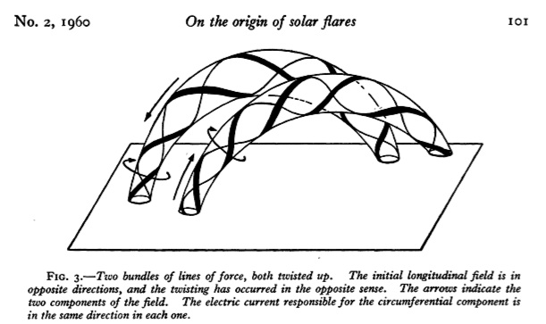
Gold and Hoyle's figure 3 showing two stable, current-carrying chromospheric plasma loops which happen to attract one another, and which later will reconnect. (Attraction will occur 50% of the time, if random). The individual tubes are energized via twisting motions in the (sub-) photospheric footpoints.
The details of their specific hydromagnetic model, consisting of two
interacting (but individually stable) twisted tubes of magnetic flux, are
perhaps not quite as long-lasting as the more general statements made
above. There is perhaps one important exception, namely that
because chromospheric plasma is partially ionized,
the ion-neutral collisions significantly enhance the resistivity
(Cowling 1947).
The dissipation of current systems might proceed at a rate
more compatible with flare observations, although Parker (1963) noted that a more careful study of
the multi-fluid equations of motion was needed to confirm that pressure
gradients would not hamper the dissipation expected. Their
model also did
not require the very thin current sheets of Sweet, Parker and others.
 D. E. Osterbrock. |
In 1961,
building upon the early work of Alfvén,
Schwarzschild and Schatzman
, Osterbrock (1961) re-investigated
MHD waves
through the solar chromosphere into the corona. Several important
advances had been made since this early work which prompted Osterbrock
to re-examine wave motions as a way of transporting and depositing
heat in the chromosphere and corona. Such advances included theories
for the generation of sound by turbulence, for shock waves and in the
theory of dissipation of waves.
His investigation is important in that it collects much of the essential physics and describes the waves and the various processes in clear physical terms. The quantitative results are less important because the assumption of near-homogeneity of the magnetic field of the solar convection zone and atmosphere was later found to be a poor description of the real Sun (Stenflo 1973). Inhomogeneity introduces a wide range of new phenomena (different wave modes, field line curvature effects,..) and qualitatively different regimes of wave dissipation, which arise because dissipative effects associated with small scales depend on wavelengths and hence the assumed Alfvén speeds. |
Osterbrock collected a variety of observational clues, both from solar and stellar data, to argue that
"...there appears to be a close connection between the solar magnetic field and the outward-propagating disturbances in the upper chromosphere".
From a theoretical point of view, he argued that MHD (wave) effects must become important somewhere within the chromosphere because
"...the velocity of sound is, to a first approximation, constant, while the Alfvén-wave velocity increases rapidly outward, because of the outward decrease in density." Osterbrock's approach was to adopt a mean (1D) atmospheric model, recognizing however that fluctuations clearly exist. He adopted radiation losses from H-, continua of hydrogen and lines of H and other species measured in chromospheric flash spectra. His estimate of total chromospheric radiation losses, to be balanced by MHD wave dissipation, was
This number exceeds coronal energy losses in the table given earlier by a factor of 30 or so. It is not dissimilar from much more modern estimates, for example Anderson & Athay (1989) give
Since fast modes in the convection zone are effectively acoustic modes, Osterbrock adopted the Lighthill-Proudman (low mach number, acoustic) approximation to compute the rate at which fast mode waves are generated there. Noting that the theory is very non-linearly dependent on the turbulent velocity, he argued that experimental work provided some justification for the theory he used, and concluded that the upward flux of sound waves is remarkably similar to his chromospheric loss estimate. Furthermore, the spectrum of wave power generated should be quite flat but with a broad peak near 0.01 Hz.
Osterbrock proceeded to calculate the generation of fast modes via turbulence in the presence of a uniform magnetic field, and their propagation using the ray approximation, but with account taken of turbulent scattering and reflection from stratification. Next he estimated Joule and ion-neutral frictional heating, and then shock formation and mode conversion.
His detailed results are somewhat academic given the extreme inhomogeneity of magnetic fields in the Sun, but the paper is full of insightful physical discussions, much of which are valid today. The inhomogeneous surface magnetic fields have prompted the study of waves in different geometries .
Resistive MHD instabilities were studied by Furth, Killeen and Rosenbluth (1963), in the neighborhood of an "X-type" neutral point. They identified three modes, the most important of which is the "tearing mode", the others being dependent upon gradients in resistivity and density. The mode can lead to break up of the current sheet, of thickness δ, into parallel current sheets along the original sheet, with a growth time (fastest modes) of the harmonic mean of the diffusion and Alfvén crossing times applicable to the sheet thickness δ:
In the particular case of a current sheet in a steady state formed by the Sweet-Parker mechanism, &deltasp=L/√RM. For a sheet thickness x δsp where x >>1
In this regard the authors noted that the MHD approximation and standard treatment of Ohm's law (neglect of ion dynamics) are formally invalid - the development of the discontinuities naturally leads to "finite Larmor radius" effects meaning that the plasma stability will ultimately depend on non-MHD effects.
The relatively large length scales associated with the linear phase of these instabilities, greater than the sheet thickness, prompted Parker (1994) (p. 11) to point out that the tearing mode instability does not change the essential conditions for formation and dissipation of current sheets via the fast topological dissipation mechanism. The rapid approach to tangential discontinuity halted ultimately by dissipation through a resistive instability is the same in ideal and resistive plasmas, justifying his approach to the coronal heating problem using ideal MHD, counter-intuitive as this may seem. In his picture the non-ideal processes are implicit.
In the period 1958-1963, considerable anxiety over the discrepancy between the Sweet-Parker rate and the more explosive behavior of flares was expressed, culminating in an article by Parker (1963), writing in 1962:
"The observational and theoretical difficulties with the hypothesis of magnetic-field annihilation suggest that other alternatives for the flare must be explored."
 Harry E. Petschek. |
In 1963, in an effort to see if the Sweet-Parker reconnection rate could be somehow increased to try to account for solar flares, Petschek re-examined the model, noting three important things: first, in their model the entire length L of the diffusing layer is needed to reconnect the field lines; second, because reconnection is a topological process, a model with a shorter L can be just as effective at cutting field lines as one with the Sweet-Parker length scale; thirdly, he examined the possibility that waves might be used to serve instead of diffusion as a way to move the frozen-in fields at a faster rate around the X-type neutral point. If a way could be found to alter the diffusion region geometry such that L' < L, the reconnection speed VR would become faster, so that mass conservation gives VRL' = VA δ, and the Sweet-Parker solution would become |
VR = (L/L')1/2 VA/ √RM.
This rate could therefore be a factor (L/L')1/2 faster than the Sweet-Parker rate.
L' is a free parameter in Petschek's model. How to make L' << L? Petschek used the idea that waves can be important to build a stationary picture analogous to Sweet-Parker's as shown:
The Petschek modification of the Sweet-Parker picture.
In this model slow mode shock waves are used to accelerate plasma to VA in the region L' < x < L . Petschek chose L' to be the maximum value allowed before currents at shock wave fronts induced magnetic fields in the reconnection region which were of the same magnitude of the reconnecting fields there. For this choice of L',
VR ≅ VA / ln RM, and
tPetschek ≅ ln RM L/VA,
Much debate over the years has focused on whether the Sweet-Parker or Petschek rates were the right ones. A re-examination of the Sweet-Parker vs. Petschek models by Kulsrud in 2000 revealed that Sweet-Parker is the correct model for constant magnetic diffusivity, but that Petschek-like behavior can arise under conditions where anomalous resistivity is important (current-driven instabilities).
 T. G. Gold, later in life. |
Gold (1964) originated the idea that the corona might be heated by field-aligned electric currents. To this end, he examined conceptually the differences between two hypothetical atmospheres: in both models, the sub-photospheric layers are in a regime where the gas dynamics dominates and the high electrical conductivity there forces the magnetic fields into a turbulent state. In the outer layers, the two models differed in that the first was insulating, the second highly conducting. The intervening surface provided the boundary conditions for the higher layers - in the first case the overlying atmosphere contains just potential fields. In the second, current systems are induced as the photospheric convection deforms and winds up solar surface magnetic fields, continuously increasing the magnetic free energy in the upper layers. He argued that the twists may become sufficiently tight that dissipation must occur, perhaps driven by dynamic instabilities. This may then account for the higher emission seen in plages overlying magnetic regions, and the high temperatures of the corona. This is the first time the idea that continuous, non-periodic changes to large scale fields may provide the energy to account for coronal heating. The central notion is a gradual build-up and sudden release of magnetic free energy in the conducting atmosphere. The energy takes the form of field-aligned electrical currents. |
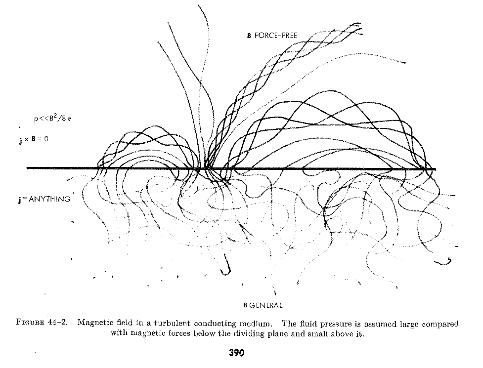
Gold's (1964) figure 2.
The above figure shows conditions in a turbulent, highly conducting fluid separated by a horizontal plane dividing regions of low and high plasma β. In contrast with a similar figure in which the upper half is an insulator and therefore occupied by potential fields, magnetic energy is stored in the force-free fields in the upper half, because the medium supports electric currents driven by conditions at the boundary plane. This picture is similar to, but also stands in contrast to Alfvén's (1947) proposal, which although driven by the same turbulent motions, considered only oscillatory motions without the new facets introduced by including steady currents caused by secularly changing twists in the magnetic field.
| Note... |
The dividing plane of course corresponds to the solar chromosphere, if observations of the solar photosphere are used to derive conditions at the top of the lower half. In this context, Gold pointed out that the difference between the potential and force-free fields in that, in the former case, all of the non-potential energy must be dissipated within the plane in order for the field to become potential above it. For force free conditions, just some fraction of the energy is dissipated there. In this way we see clearly that the electrodynamics of the chromosphere is critical to the supply of magnetic free energy into the corona. |
Parker envisaged a model of the Sun's corona as a conducting fluid between two infinitely conducting "plates", which represent two separate ares of the solar photosphere. The footpoints at one of the plates move with a random motion approximating the dynamics of convection cells (granules).
Sweet (1958) had noted that neutral points represent a non-equilibrium state, leading to dissipation of magnetic energy in a diffusion region. Prompted by this, Parker studied the above picture and concluded that turbulent convective photospheric motions drive the corona into a state for which force balance cannot be met while, so that the magnetic field is again expected to relax dynamically, but under quite different conditions. Parker concluded that the dissipation must result because there exist equilibrium states only under artificially contrived conditions which are characterized by symmetries unlikely to be found in nature. The result was that the subsequent evolution would be dynamic. Parker referred to this process as "topological dissipation".
This particular claim has since proven incorrect, as shown analytically by van Ballegooijen (1985) and confirmed in later numerical work. Non-potential equilibria do exist in non-trivial geometries, the magnetic stresses being taken up by the boundaries. The tangential discontinuties are not obliged to dissipate in the manner argued by Parker. Instead equilibria are maintained by the boundary stresses, so Van Ballegooijen showed that any discontinuities present in the coronal volume must also be present at the boundaries.
|
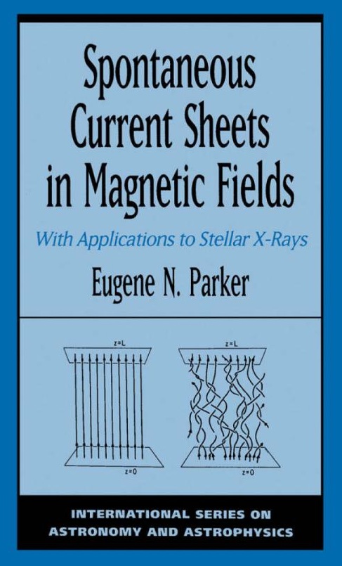
Nevertheless, Parker's work is important in highlighting the formation of tangled or "untidy" magnetic fields, which contain small scale structures, in response to granular motions. The inevitability of this process with accompanying dissipation was elaborated on in Parker's (1994) monograph, Spontaneous current sheets in magnetic fields with application to stellar X-rays. The fundamental idea is that a highly conducting MHD fluid, subjected to boundary motions determined by turbulent processes, will inevitably develop tangential discontinuities within the volume, which will dissipate via processes probably outside of the MHD approximation. Another way of saying this is that the field topologies expected in the Sun (and other natural physical systems) are generally incompatible with field continuity. Tangential discontinuties must form. This body of work again related the dissipation of magnetic energy to field line topology, but in a less orderly fashion than discussed by Kruskal and Kulsrud (1958), for example. Hahm & Kulsrud (1985) found that a magnetic field, initially force-free, could evolve linearly in response to an infinitesimal change of shape of its domain, by seeking a new equilibrium containing a current sheet. This result was generalized by Low (2006, 2007), who has given examples of 3D untwisted fields, anchored at a boundary, which are unable to obtain a force-free equilibrium in the absence of current sheets. The absence of twists which are central to parker's theory, but the formation of sheets, represents a new mode in which current sheets are formed spontaneously as a result solely of fixing the connnectivity of magnetic footpoints. It points to the inevitable formation of current sheets in general, untwisted geometries, indicating that such sheets might be ubiquitous and hence forming a dense population of current sheets in most astrophysical plasmas. |
|
 J. Bryan Taylor, winner of the 1999 James Clerk Maxwell Prize for Plasma Physics. |
In 1974, Taylor explained how the generation of reversed fields observed in toroidal plasmas arises because the plasmas relax under certain constraints. The work is of much broader importance than the specific application he studied, Taylor showed that the well-known result of the "frozen flux" condition in the ideal MHD equations is expressed simply through the "magnetic helicity" K which, in the limit of infinite conductivity, is conserved, for a volume V bounded by field lines:
Then, it is easy to show with vector identities and integration by parts that, provided a volume V is bounded by field lines, magnetic surfaces, or B→0 at infinity, then |
Thus, when the constraint of constant magnetic helicity is applied to an ideal magnetofluid, the system will evolve to a state of minimum energy where the constant α may be different for all field lines. In this case the exact minimum energy state to which the fluid will evolve will be determined by the initial values of the invariant quantities K for all the field lines.
Taylor took the argument a step further by examining the consequences
of permitting finite conductivity in the fluid. When effects due to
resistivity are permitted (or other effects due to inertial terms,
plasma instabilities,
turbulence or anomalous resistivity), field lines can break so that a
topological invariant such as K has no meaning for individual
lines of force. Noting that changes in field topology are often
accompanied by very small changes in the field itself (such as in
Sweet-Parker reconnection), Taylor argued
that the effect of the topological changes is "merely to redistribute
the integrand among the field lines involved". The final relaxed
state will thus be the minimum energy state subject to the single
invariant
for the entire fluid volume V0. Woltjer (1958) had shown earlier that the lowest energy state accessible to this system is that which has a constant α throughout the system
Taylor's work has been extended to considerations of the solar corona (e.g., Berger 1984). He argues that the dissipation of helicity occurs at a far shower rate that that of energy, so that the conservation of magnetic helicity limits the available equilibrium states. Care must be taken to include sources and sinks of helicity from the lower atmosphere and into the heliosphere, which prevent the corona from being treated as a closed magnetic system.
Interestingly, by considering the global magnetic solar helicity, Low (1994) has made a case for a Sun whose magnetic helicity plays a central role in the solar magnetic activity cycle: coronal mass ejections are needed to shed the magnetic helicity generated each 11 years.
The introduction of non-trivial geometry into the solar magnetic structure has profound implications for the magnetohydrodynamics, even in the case of magnetostatics, as symmetries are broken. One area of special interest for the coronal heating is the modification of wave motions which can occur.
Progress in this area has therefore been made in steps, as more and more assumptions are relaxed, for example:
 Peter Wilson, Sydney University. |
A natural first step was to examine simple geometries under conditions of planar and cylindrical symmetry. Peter Wilson was one of the first to deal with waves in structured magnetic fields in the solar context. With Lawrence Cram, in 1975 he studied the propagation of plane waves across semi-infinite magnetic and non-magnetic domains. His short report Hydromagnetic Waves in Magnetic Flux Tubes (1977) is the first to address wave modes of a magnetic flux sheath or tube (plane slab or cylindrical symmetry) including the coupling of waves at the magnetic/non-magnetic interface. (Earlier work by Defouw (1976) did not include this important effect). In the limit that the wavelength greatly exceeds the wavelength (a "thin flux tube" approximation for a non-stratified medium) he discovered that the dispersion relations were the same in both geometries, for the two modes he considered: pulsation modes and taut-wire modes. Initially, there was debate with Roberts and Webb concerning the appropriate expansion procedure for small perturbations which was later resolved (Wilson 1980, Roberts & Webb 1979). |
 Prof. Bernard Roberts, University of St. Andrews. |
The lowest (m=0,1) azimuthal orders of these "tube" or "body" magneto-acoustic modes were termed "sausage" and "kink" modes (Edwin & Roberts 1983). These authors and Edwin, Roberts & Benz (1984) examined the properties of the modes under coronal conditions. Shear "Alfvén waves" in these geometries exist trivially within and outside of the cylinder, their dispersion relation and hence mode being decoupled from the magneto-acoustic case as for homogeneous plasmas. |
 James Ionson, formerly U. Maryland and later lead scientist of the US Innovative Science and Technology Directorate of the SDI program. |
In 1978, Ionson proposed a model for heating active region loops with two new ingredients: irreversible heating by surface Alfvén waves and energy transport via an induced boundary-layer convection. "Surface waves" are those natural oscillations which owe their existence to the presence of inhomogeneities in the background medium, and they become more important relative to the familiar "body" oscillations as the scale of the inhomogeneities decreases. For discontinuous inhomogeneities, the waves become pure surface waves analogous to those on the surface of a lake. Ionson's particular model was inspired by SKYLAB observations of a class of relatively cool loops (104 - 2 ×10⁶ K) originating in sunspots, which were inferred to have a sharp radial dependence of temperature with loop radius by Foukal (1975). The sharpest loops were coolest and located at the loop axes, with progressively hotter loops being seen farther from the axes. In 1976, Foukal argued that the cool material originated from cross-field flow at hot loop tops, and was condensing from the hotter material and falling under gravity. |
The essential property leading Ionson to examine the resonant absorption process was the apparent gradient in Alfvén speed with radius from the tube axes. This is because in an inhomogeneous ideal plasma there exist two continuous parts to the spectrum of natural oscillations: the Alfvén continuum and slow magnetoacoustic continuum. Ionson's first ingredient exploits the fact that the a given Alfvén wave can couple to the Alfvén continuum and produce a resonance whenever the wave phase speed equals the local Alfvén speed. This phenomenon was proposed as a mechanism to enhance heating in plasma devices (e.g., Hasegawa & Chen 1974), where the drop of resistivity with temperature due to Coulomb collisions limits the temperatures otherwise attainable. In cylindrical symmetry, the radial and tangential plasma velocity components possess singularities under this condition. The wave energy is thus fed into a thin layer around this point until non-linearities or dissipative effects take over. Eventually, if dissipation dominates, a stationary condition can be achieved in which all wave energy is thermalized and the power of an external driver is exactly balanced by the energy dissipation rate.
Ionson's original work focused on accounting for the particular thermal properties inferred by Foukal, hence he included his second ingredient as a special case, and invoked the resonant absorption to explain the hottest, outermost shells of coronal emission associated with the observed loops. Subsequent convection and an electrostatic instability at the loop apex was then used to explain the plasma seen on the loop axis.
 |
However, because the solar corona is not homogeneous, and the active corona appears to be highly filamentary in nature, the resonant absorption process remains of more general interest. Hollweg (1987) was able to reduce the mathematics of resonant absorption to a relatively simple physical picture in which pressure perturbations drive velocity perturbations in a fashion analogous to a driven classical oscillator, through:
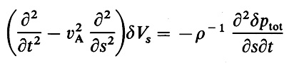
|
Here, s is distance along a magnetic field line, VA the Alfvén speed, δVs the velocity fluctuation at s, ρ the density, and δptot the total (gas plus magnetic) pressure perturbation, seen here as a driving term. Hollweg goes on to show that the resonance condition can be relaxed. Two adjacent waves are approximately in resonance provided that the phase difference, over the time it takes for the energy to be transformed from the driver into the energy containing resonance layer, is small. In this way he shows that the thickness of the resonant layer scales as ka2 where k is the wavenumber and a is the characteristic scale length of the inhomogeneity. If the subsequent evolution of the resonant layer oscillations is dissipation (via viscosity or Joule heating, for example), then the wave energy dissipation rate becomes independent of the dissipation process: the width of the resonant layer adjusts itself to dissipate the energy independent of the thermalization process:
Ionson originally invoked kinetic properties of the driven Alfvén continuum oscillations to allow dissipation, a curious situation since his work started from ideal MHD. This point has since been clarified (e.g., Lee 1980) and Ionson's attribution of the transfer of energy as dissipation was shown to be incorrect. Instead, one must invoke genuine irreversible processes involving collisions between particles (described by dissipative transport coefficients in the case of fluids).
The ultimate fate of the energy in the resonance layer and fate of the whole scenario is debated still. Nevertheless the process has several properties in its favor:
Primary difficulties with the mechanism are
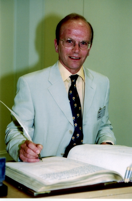 Eric Priest FRS, 2002 Hale prize winner. |
Observations of the upper chromosphere showed that the slow-modes were already known to carry insufficient energy flux to heat the quiet corona. Similar amounts of energy were estimated to drive the fast solar wind from coronal holes. Van de Hulst in 1951 showed that Alfvén waves suffer very weak damping due to Joule and viscous dissipation. Only in partially ionized plasma would ion-neutral frictional damping be significant (i.e. Cowling's (1945) "transverse conductivity", as invoked under special conditions by Gold & Hoyle 1960). By 1983, the problem of heating and driving the solar wind was to identify a way to dissipate Alfvén-type and fast-type waves effectively within coronal plasma, assuming that such waves would originate from the highly turbulent photosphere, as originally suggested by Alfvén (1947). Heyvaerts & Priest (1983) noted that shear Alfv\eacute;n waves propagating along adjacent field lines can have different phase speeds if the phase speeds are different in the direction normal to the plane of polarization of the waves. As such waves propagate (or as time proceeds in the case of standing waves) they become more and more out of phase, leading to large shears and steep gradients in wave fronts which become more and more corrugated with time. In this way, they argued, wave energy might be converted by instabilities into ultimately via Joule or viscous dissipation. |
Coronal holes contain what appear to be density enhancements aligned along magnetic fields. Such inhomogeneities are evident in historic pictures of the corona during eclipse as rays (e.g., Young 1896), as well as modern white-light measurements. Thus, gradients in Alfvén speeds certainly exist at the lower regions of the solar wind, and phase mixing should be expected, and Heyvaerts and Priest argued that such effects will be important in the Sun.
There is a catch, however. Parker 1991 showed that phase mixing can only occur under more special conditions of inhomogeneity than are likely to be found on the Sun. Phase mixing requires that the waves propagate in a medium with an "ignorable coordinate" in the geometry such that the Alfvén and other waves are effectively de-coupled. Heyvaerts and Priest used the following equation to describe the wave motions, derived from linearizing the non-ideal MHD equations with variations along cartesian axes x, z but not y:
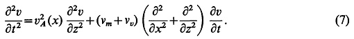
Here, z is the field direction, y the direction of polarization of the Alfvén wave displacements. A crucial assumption is that v=(0,vy,0). This equation leads to strong phase mixing because the different planes x=constant can oscillate independently. This equation stands in contrast to the more general (but ideal) form discussed by Parker 1991, who permits oscillations in v in all three coordinates. In words, phase mixing requires inhomogeneity but also symmetry, such as may be found only under special circumstances such as cylindrical flux-tube geometries, or in the limit where wavelengths are less than the length scales of the coronal inhomogeneities.
Waves of some kind - the simplest being Alfvénic- must be present to account for the properties of coronal holes as compiled by Withbroe (1988). A total energy flux of 4-8 ×10⁵ erg cm-2 s-1 is needed to balance energy losses due to radiation, conduction and in accelerating the wind. To account for conductive, radiative losses and the mass flux, most of this energy must be deposited in the flow within the first 1-2 solar radii above the solar surface. To account for the high speed wind streams, additional energy (say 20% of the total) must be deposited at several solar radii.
In the first paper, Parker re-assesses the viability of Alfvén waves as the agent through which the solar wind can be driven, assuming that a suitable wave flux generated in the (sub) photosphere exists. Parker examines how a general lack of symmetry might affect the wave propagation and in particular the phenomenon of phase mixing in the corona. In contrast with the work of Heyvaerts & Priest (1983), Parker includes spatial derivatives in 3 cartesian coordinates, concluding that phase mixing requires special conditions unlikely to exist in the corona. Parker's three linearized equations (his equations (10)-(12)), including non-zero derivatives in three spatial coordinates, produce coupling between the previously independent oscillations found by Heyvaerts & Priest (1983), such that no phase mixing is possible. Phase mixing requires there to be no coupling between different planes of polarization of Alfvén waves, which is not possible except when specific gradients are negligible. Parker shows in his section 3 a specific example where inclusion of oscillations along the magnetic field as well as in the plane of polarization couples the velocities in these directions. The coupled waves are sometimes called "coordinated modes".
An important characteristic of coordinated modes is that they have a specific relationship between wavenumber and frequency. ???
In the paper " Heating solar coronal holes", Parker assesses the viability of Alfvén waves as drivers of the solar wind (and of heating the quiet Sun). Focusing on generation and dissipation mechanisms, Parker surveyed the known physics of solar plasmas. He concludes that
"the necessary Alfvén waves are not produced under the conditions presently known to exist in the Sun [i.e. the photosphere], nor would such waves dissipate significantly in the [required] 1-2 Rsun if they existed".
By elimination, and prompted by the suggestion of Martin (???, 1984), Parker is then led to identify the sources of Alfvén waves with the continuous activity of the small-scale magnetic fields which are associated with the chromospheric network, forced by granular and supergranular motions to reconnect within the chromosphere thereby releasing energy in the form of heated plasma, plasma flow and wave motions into the corona.
The same ideas were later adopted by others, e.g., Axford and McKenzie "The origin of high speed solar wind streams" in Solar Wind Seven; Proc. 3rd COSPAR Colloquium, pp. 1-5 (1992). This scenario was later dubbed the "magnetic carpet" by Title and Schrijver in the context of quiet Sun as well as coronal hole plasmas ("The Sun's Magnetic Carpet", ASP Conf. Ser. 154, The Tenth Cambridge Workshop on Cool Stars, Stellar Systems and the Sun, Edited by R. A. Donahue and J. A. Bookbinder, p.345, 1998).
 Paul Bellan, of Caltech |
In 2003, Paul Bellan
addressed the problem of why some coronal plasma
loops do not seem to expand with height, in particular those observed
with the TRACE spacecraft. If bright coronal plasma loops correspond to
tubes of magnetic flux generated largely by sub-photospheric electric
currents,
then the loops would be expected to expand with
height in the corona according to solutions of Laplace's equation.
Clearly then, either the observed structures do not delineate such flux tubes,
or the magnetic fields are not close to a potential type. Bellan examined the case of a bulging cylinder containing plasma with a small but finite values of the plasma β, in which axial ("poloidal") currents are slowly introduced and maintained. Bellan replaced the coronal loops with cylinders, ignoring gravity, but allowing for tube expansion, under the assumptions of rotational symmetry around the axis and reflective symmetry about the axis mid point (z=0). Thus the initial state considered by Bellan is given by figure labeled (b) below: |
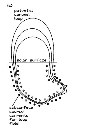
Bellan's (2003) figure 2a. |
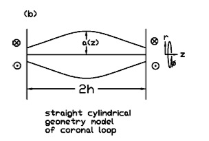
Bellan's (2003) figure 2b.
His analysis started with a potential field and equilibrium (constant pressure) plasma. He considered a twist at one footpoint leading to an axial electric current which varied from zero to a finite value with a steady rise on timescale τ. Bellan argued that the dynamics will proceed in three phases:
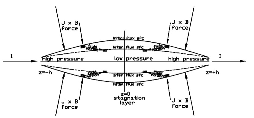
Bellan's (2003) figure 5.
Bellan supposes that the final state is one where the loop tops are over-pressured with respect to the footpoints, they have a higher toroidal/poloidal magnetic flux ratio, and the tubes become straight.
It should be noted that
 Dr. T. Arber of Warwick University |
Through the 19th and early 20th centuries it became clear that the quiescent corona had to be close to a force-free equilibrium state. This was evident simply because of the apparent dominance of magnetic forces in the corona which cause coronal emission features (loops, plumes, prominences) to appear to follow magnetic lines of force. In general, the transition from forced to force-free takes place in the partially ionized photosphere and chromosphere (see the note after Gold's (1964) discussion). Thus, on the basis of force balance alone, the chromosphere contains the β=1 surfaces near which the systems adjusts from a forced to a near-force free state. But, this is only part of the story. In 2006, Leake & Arber (2006) showed that ion-neutral collisions within the chromosphere tend to dissipate cross-field currents before they reach the corona. Using 2.5D numerical simulations of flux emergence through the entire atmosphere, they found that the resistivity calculated by Cowling tended to dissipate cross field currents generated in the convection zone and photosphere before they reach the corona. In later work, Arber, Haynes & Leake (2007) investigated the same problem in 3D, finding similar effects at the microscopic level but some other interesting phenomena related to it, associated with the larger scale dynamics. The inclusion of Cowling's conductivity was found to lower the amount of mass which the Lorentz force could lift to coronal heights, such that treatments omitting it would over-estimate the mass supllied to the corona. |
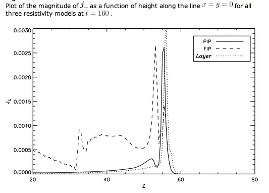
Arber, Haynes & Leake's (2007) figure 2 . The figure shows the perpendicular current through the model chromosphere as a flux tube emerges through the surface, along one vertical locus in their calculation. The "PIP" (partially ionized plasma) calculation includes cross-field dissipation, the FIP calculation (fully ionized) does not. (The "layer" calculation is a simple height- and magnetic field- dependent parameterization of the cross field resistivity). The cross field dissipation makes the perpendicular current approach zero at the base of the corona.
Earlier work by Goodman had shown that the dissipation of wave energy through the chromosphere via the Cowling resistivity may explain the large amount of heating necessary to maintain the chromosphere against radiative and other losses.
Clearly, this work re-emphasizes the importance of understanding the detailed physics of the chromosphere, prior to being able to study effectively the coronal heating problem.
While flares were recognized in the 1940s as requiring magnetic energy, the favored heating mechanisms of the corona until the 1970s was the dissipation of acoustic waves. This is a little surprising given that the magnetic nature of the corona seen during eclipse had been apparent to observers already by 1900. In the 1960s and 1970s, X-ray data from space had revealed this yet again, showing concentrations of X-ray emission on a variety of scales on the solar disk, and their association with surface magnetic flux concentrations. The observed magnetic structuring of the X-ray corona seemed inconsistent with a turbulent, acoustically heated atmosphere.
During this "renaissance", Levine (1974b) was one of the first to take seriously the idea that the quiet and active corona, as well as flares, is heated by magnetic processes. The particular process Levine advocated was the acceleration of ions (mostly protons) from a thermal distribution (Levine 1974a) by extracting energy from the kinetic energy of matter frozen to converging magnetic fields of the kind considered by Dungey (1953), during the contraction phase of X-point reconnection. As Dungey argued, such neutral points automatically attract opposite polarity fields via the Lorentz force. The motions of the attracting fields serve to accelerate particles lying between them. Levine requires not the steady state represented by the Sweet-Parker model, but to the dynamic, formation phase of a neutral sheet.
Levine's physical model is a modification of the Fermi (1949) process proposed to accelerate cosmic rays to GeV and higher energies. Levine argued that protons are accelerated during the collapse phase and that their subsequent coulomb collisions with particles dumps energy in the ambient atmosphere. The X-ray images might correspond to the ambient corona heated by neutral sheets of X-point reconnection sites.
Like Fermi's theory, Levine's scenario requires the existence of some particles within the neutral sheets as a seed. For conditions in the interstellar medium, Fermi found that an injection of particles already at a relatively high energy (200 MeV) was needed to get the process started. Levine's model just required the presence of some ionized plasma particles is all that is needed for net acceleration to occur. Formation of a hot corona seems inevitable provided the energy gains exceed the losses due to particle collisions. Given the large coronal mean free paths for coulomb collisions, conditions for acceleration appear favorable for rapidly collapsing neutral sheets. Levine's (1974a) equation (51) shows that for acceleration the collapse time of the neutral layer tB must obey
where T is the temperature in K and n the proton density in cgs. For the corona, this is 15 seconds. Hence this picture requires the rapid and continual formation of neutral sheets throughout the corona.
Alfvén, H., 1942, "Existence of electromagnetic-hydrodynamic waves", Nature 150, 405
- Also
Goodman M. L., 2001. "The Necessity of Using Realistic Descriptions of Transport Processes in Modeling the Solar Atmosphere, and the Importance of Understanding Chromospheric Heating", Space Science Reviews, 95, 93-79
Goodman M. L., 2004. "On the efficiency of plasma heating by Pedersen current dissipation from the photosphere to the lower corona", A&A, 416, 1178-1159
Goodman M. L., 2004. "On the creation of the chromospheres of solar type stars", A&A, 424, 712-691
Kazeminezhad F., Goodman M. L., 2006. "Magnetohydrodynamic Simulations of Solar Chromospheric Dynamics Using a Complete Electrical Conductivity Tensor", ApJS, 166, 633-613
Low, B.C., 2007, "On the possibility of electric-current sheets in dense formation", Physics of Plasmas, 14, 122904 citation in text