Do it yourself script examples

Polar Stereographic Plots

polar_1.ncl: Default black and white plot. gsn_csm_contour_map_polar is the plot interface that creates a cylindrical equidistant plot. cnLineLabelPlacementMode = "constant", is one of the three methods for controlling contour labels. the constant method is the only one in which the label becomes part of the line. There are four title strings you can use to label a plot. The gsnLeftString is automatically labeled with the long_name of the data, and gsnRightString is labeled with the units of the data. These can both be overwritten, or turned off (by setting them to ""). There is also gsnCenterString and the plot title tiMainString. res@mpMinLatF and res@mpMaxLatF are used to limit the extent of the plot in the southern and northern hemisphere respectively. gsnPolar allows you to choose a hemisphere. The default is the nothern hemisphere.

polar_2.ncl: Adds color and a local time axis. cnFillOn = True, turns on a color plot. gsnSpreadColors is a special resource that tell the plot template to use the full range of the colormap. There are many built-in colormaps to choose from and many ways of specifying the color of a plot. ZeroNegDashLineContour is the special shea_util.shtml function that will take contours and make the zero line double thickness, and the negative lines dashed. There are many other contour effects you can use. gsnPolarUT and gsnPolarTime turn on the local time on a polar plot.

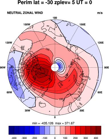
polar_3.ncl: Manually sets contour levels, turns on contour labels, and puts the min/max of the data on the plot. cnLevelSelectionMode = "ManualLevels" cnMinLevelValF cnMaxLevelValF cnLevelSpacingF are the resources that manually sets the contour levels. The NCL built-in functions min and max allow you to take the min and max of the data. cnLineLabelsOn = True will turn on the contour line labels. These are turned off by default on color plots.

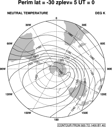
polar_4.ncl: Demonstrates a panel plot. There are too many nuances associated with panelling. Please review the CCSM panel example page for details.

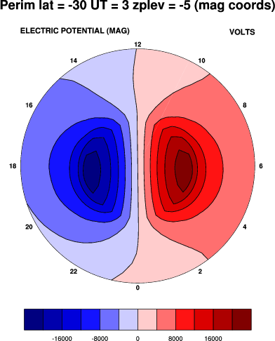
polar_5.ncl: Demonstrates plotting data on magnetic coordinates The function mag2latlon (found in hao_cobntrib.ncl takes data on magnetic coordinates and changes the named dimensions fixes the units of the coordinate variables so that the NCL gsn_csm plot interfaces do not produce error messages. It is necessary to turn off the cyclic point by setting gsnAddCyclic to False. The gsn templates automatically add a cyclic point, and data on the magnetic coordinates already has one. mpGridAndLimbOn turns on the grid lines.

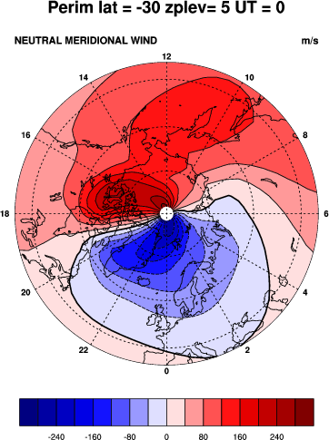
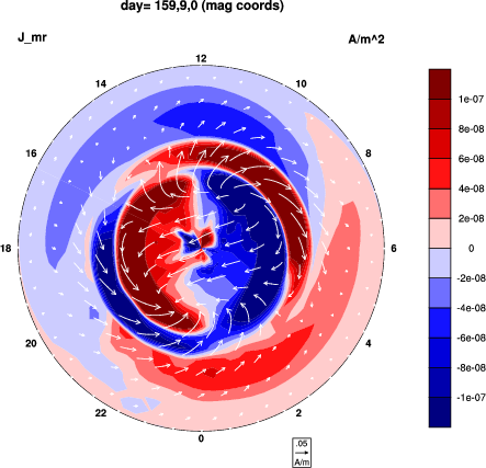
polar_6.ncl: Adds vectors and explicit contour levels. To effectively view the variable in this example, it was necessary to explicitly set the contour intervals. This is done with cnLevelSelectionMode = "Explicit" and providing values to cnLevels. This example draws vectors on top of scalars. For a complete description of the vector resources used, and other vector options, please check out the CCSM vector page

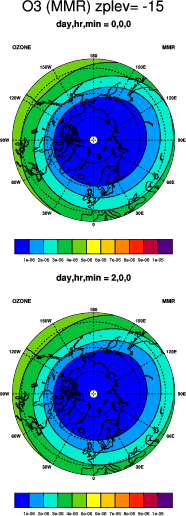
polar_7.ncl: Demonstrates interpolating the data to height before plotting.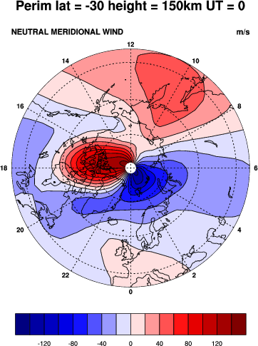 hao_contrib.ncl contains the function "zplev_to_height" which we use to interpolate to height in the master scripts. Note that this function requires the create of a logical variable to which you attach the height value. In the master scripts this variable is also used for other things.